

 journal menu


research papers
 | JOURNAL OF APPLIED CRYSTALLOGRAPHY |
Correlation-aware binning for small-angle neutron scattering via Gaussian-process inference

aNeutron Scattering Division, Oak Ridge National Laboratory, Oak Ridge, TN 37831, USA, bNeutron Science Division, Korea Atomic Energy Research Institute, 989-111 Daedeok daero, Yuseong gu, Daejeon 34057, Republic of Korea, cDepartment of Engineering and System Science, National Tsing Hua University, Hsinchu 300044, Taiwan, dPhysics Division, National Center for Theoretical Sciences, Taipei 10617, Taiwan, eInstitut Laue–Langevin, BP 156, F-38042 Grenoble Cedex 9, France, fCenter for Nanophase Materials Sciences, Oak Ridge National Laboratory, Oak Ridge, TN 37831, USA, and gMaterials Science and Technology Division, Oak Ridge National Laboratory, Oak Ridge, TN 37831, USA
*Correspondence e-mail: [email protected], [email protected]
This article is part of a collection of articles related to the International Conference on Neutron Scattering, ICNS2025.
Binning in small-angle neutron scattering (SANS) is typically performed empirically, with fixed parameters chosen for convenience rather than statistical optimality. Such practices often fail to balance statistical precision and spatial resolution, leading to inconsistencies across instruments and datasets. Here we establish a correlation-aware framework that determines the optimal bin width from first principles by extending the classical Freedman–Diaconis (FD) rule to account for inter-bin correlations with a Gaussian process. In this formulation, the scattering intensity is treated as a smooth stochastic field whose statistical coherence is described by a covariance matrix. Analytical expressions of errors derived from this model yield closed-form criteria that separate the total deviation into contributions from counting noise, aliasing distortion and curvature-dependent correlation effects. Expressed in reduced variables, the resulting dimensionless error surface reveals a continuous transition from the uncorrelated FD regime to the correlation-dominated limit, providing a unified description of noise suppression and resolution control. Because the formulation depends only on the profile characteristics of scattering intensity I(Q), specifically its average intensity and first- and second-order derivatives, it applies generally to any SANS measurement regardless of sample, instrument or geometry. Experimental validation using small- and ultra-small-angle neutron scattering data confirms the predicted scaling behavior, demonstrating that correlation-aware inference systematically reduces mean-squared error and enables information-efficient reproducible data reduction across materials and instruments.
Keywords: small-angle neutron scattering; SANS; ultra-small-angle neutron scattering; USANS; Gaussian-process regression; binning.
1. Introduction
Small-angle neutron scattering (SANS) is a widely used technique for probing nanoscale structures and correlations in soft matter, polymers and complex fluids (Lindner & Zemb, 2002 ). Measuring the scattering intensity as a function of momentum transfer reveals characteristic length scales and internal organization that are inaccessible to direct imaging. The accuracy of the reconstructed intensity profile depends critically on how neutron counts are discretized and averaged during data reduction. The binning process, which groups detector signals into intervals of momentum transfer with bin width h, governs the balance between statistical precision and spatial resolution, determining the fidelity of the measured scattering curve.
In most measurements, binning is performed with fixed or empirically chosen parameters. A single binning scheme is often applied to all datasets regardless of variations in signal strength, scattering contrast or structural complexity. Coarse binning suppresses statistical noise but obscures subtle structural features, whereas overly fine binning amplifies counting fluctuations and introduces artificial variations that do not reflect intrinsic scattering behavior. Without a statistically defined criterion for selecting h, this balance between noise suppression and resolution remains subjective, leading to inconsistencies across instruments, samples and measurement conditions.
A more systematic alternative to fixed or empirical binning is to determine the bin width from statistical principles. The Freedman–Diaconis (FD) framework (Freedman & Diaconis, 1981) provides such a foundation by balancing random counting noise against systematic averaging bias, thereby identifying the bin width that minimizes the total deviation between the discretized and underlying intensity. This approach offers a clear and objective criterion for optimizing histogram resolution and serves as a natural starting point for formulating statistically consistent binning in scattering experiments. Yet scattering data exhibit additional complexities that extend beyond the assumptions of the FD framework. In particular, the measured intensity varies smoothly and continuously with momentum transfer as a consequence of both the underlying physical structure and instrumental resolution, giving rise to strong inter-pixel correlations (Tung et al., 2025b). These correlations are inherent to SANS but have never been explicitly accounted for in the FD formulation. As a result, the FD approach cannot leverage prior knowledge about the common characteristics of realistic scattering measurements. This shortcoming motivates the development of a correlation-aware framework that explicitly incorporates the coherent nature of scattering signals.
Building on this understanding, we develop a correlation-aware framework based on Gaussian-process (GP) inference (Rasmussen, 1996; Rasmussen & Williams, 2006). In this formulation, the scattering intensity is treated as a smooth stochastic field whose statistical dependence between measurement points is described by a covariance matrix  . The kernel encodes spatial correlations through a characteristic length scale λ, which defines the range over which neighboring bins exchange information. Each observed intensity
yk at bin center
Qk is assigned by the corresponding histogram counting, and its uncertainty is determined by Poisson statistics. The posterior mean is then obtained by combining observations according to the kernel covariance and their individual uncertainties, yielding the maximum a posteriori estimate of the underlying signal. When the correlation length is short (
. The kernel encodes spatial correlations through a characteristic length scale λ, which defines the range over which neighboring bins exchange information. Each observed intensity
yk at bin center
Qk is assigned by the corresponding histogram counting, and its uncertainty is determined by Poisson statistics. The posterior mean is then obtained by combining observations according to the kernel covariance and their individual uncertainties, yielding the maximum a posteriori estimate of the underlying signal. When the correlation length is short ( ), neighboring bins act independently and the formulation reduces to the uncorrelated FD limit. For comparable or larger correlation lengths (
 ), curvature-dependent corrections arise, further suppressing noise beyond the histogram-averaged observations and revealing the coherent structure of the scattering data.
Incorporating inter-bin correlations fundamentally extends the scope of classical binning theory. By exploiting the inherent smoothness of scattering data, the correlation-aware framework surpasses the variance–bias balance of the FD rule and provides a statistically optimal description of realistic measurements. Accounting for correlation simultaneously suppresses stochastic noise and preserves structural fidelity, linking statistical inference directly to physical resolution. This framework establishes a unified predictive basis for precision binning in SANS and enables consistent information-efficient data reduction across instruments and materials.
2. Methods
Classical binning rules were developed in general statistical contexts and are not specifically tailored to the requirements of scattering experiments. To apply such methods in this setting, it is necessary to adopt a representative statistical baseline. Among the established approaches derived from probabilistic or information-theoretic criteria, the FD rule (Freedman & Diaconis, 1981) is particularly appealing for its simplicity, robustness and broad applicability. Accordingly, we take the FD rule as our reference point and first formulate an uncorrelated binning framework that reproduces its underlying variance–bias balance in a scattering context. We then extend this baseline to a correlation-aware framework based on GP inference (Rasmussen, 1996; Rasmussen & Williams, 2006), in which neighboring bin intensities are coupled through a continuous kernel. This generalized formulation yields closed-form error criteria that simultaneously account for statistical noise, aliasing distortion and inter-bin correlation, reducing seamlessly to the classical FD limit when correlations vanish.
2.1. Uncorrelated binning framework
In scattering experiments, the quantity of interest is the intensity distribution
I(Q) (Lindner & Zemb, 2002) measured over the momentum-transfer interval
[Qmin,Qmax]. Within the FD framework (Freedman & Diaconis, 1981; Scott, 1985), the quality of a histogram approximation
Ih(Q) with bin width h is assessed by its
L2 deviation (Freedman & Diaconis, 1981; Scott, 1985; Strang, 2023) from the underlying distribution
I(Q),
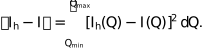
Normalizing by the interval length  gives the mean-squared deviation,
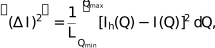
which serves as the objective function for evaluating binning performance.
In the uncorrelated framework, the detector partitions the scattering vector range into K equal-width bins of size

and records
Nk counts in bin k, with total count  . Assuming the measured intensity
I(Qk) is proportional to
Nk,
. Assuming the measured intensity
I(Qk) is proportional to
Nk,

In the continuous limit, the binning-independent normalization constant CI reduces to the mean intensity of I(Q) over [Qmin,Qmax], a quantity routinely determined in instrument calibration.
Under Poisson statistics (Knoll, 2010), the counting variance in bin k is

Approximating  , where
  denotes the bin-averaged intensity of the kth interval in the histogram estimate
Ih, and averaging over all bins gives the counting uncertainty
denotes the bin-averaged intensity of the kth interval in the histogram estimate
Ih, and averaging over all bins gives the counting uncertainty

Finite bin width also introduces a systematic aliasing distortion because I(Q) is estimated by its average within each bin. A Taylor expansion of I(Q) around the bin center Qk yields

where the prime denotes the derivative.
The total mean-squared deviation combines the independent counting and aliasing errors:

Substituting equations (4) and (5) gives
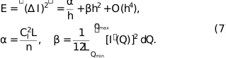
Minimizing with respect to h yields the optimal bin width,

2.2. Correlation-aware binning framework via Gaussian-process inference
We generalize the uncorrelated framework by applying GP inference to the binned data, thereby incorporating inter-bin correlations arising from detector geometry and instrumental resolution.
The essential difference from the uncorrelated model lies in how statistical dependencies between neighboring bins are represented. In the GP formulation, these dependencies are encoded in the covariance kernel , whose correlation length λ sets the characteristic scale over which variations in the scattering intensity
I(Q) are treated as statistically coherent. When , bins behave independently and the results reduce to the uncorrelated limit of equations (6) and (7). Conversely, for  , the GP prior enforces smooth, collective variation across bins, effectively coupling their fluctuations. Thus, λ provides a mathematically continuous means to interpolate between pixelwise independence and global correlation, enabling the binning process to account for both statistical and physical sources of coherence. We therefore define the dimensionless parameter
  to quantify the degree of correlation between neighboring bins.
At bin centers  ,
,

where we represent the measured scattering intensity as the sum of a deterministic mean component and a stochastic noise term, denoted by η, and we impose a GP prior with squared-exponential covariance:

Let  ,
,  and
and  . The posterior mean at the bin centers is then obtained through Gaussian-process regression (GPR) (Rasmussen & Williams, 2006)

via the operator defined as

The counting contribution to the average mean-squared error is

For equal-width bins  and locally uniform noise, the operator in equation (12) acts as a normalized, symmetric weight sequence
  , with
 and (Rasmussen & Williams, 2006). Z is selected such that
  . This leads to
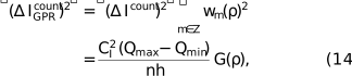
where, for the squared-exponential kernel,

and

is the third Jacobi theta function.
Using  and a local Taylor expansion about
Qk, the averaged systematic distortion becomes
and a local Taylor expansion about
Qk, the averaged systematic distortion becomes
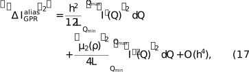
where and

Combining equations (14) and (17) gives

with
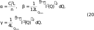
Equations (19) and (20) directly mirror the uncorrelated formulation in equations (6) and (7): the first term corresponds to the counting error modified by the correlation factor  , while the second and third terms generalize the systematic bias by introducing a curvature-dependent correction through
  . Note that this result also holds for the Bonse–Hart geometry (Bonse & Hart, 1965) to leading order, where the binned estimation converges to the underlying signal in the long-time limit.
2.3. Total deviation in reduced-unit representation
To compare different experimental conditions on a common dimensionless scale, we introduce characteristic quantities that normalize the bin width and the total error, while keeping the GP correlation ratio unchanged. Balancing the counting and bin-averaging terms in equation (19) defines the characteristic bin-width scale (in units of Q)

and the corresponding characteristic error scale (in units of I2)

These quantities represent, respectively, the bin width and the mean-squared deviation at which the variance and bias contributions become comparable.
We then introduce reduced (dimensionless) variables

which express all results in terms of normalized quantities independent of experimental units.
To incorporate the curvature term introduced by GP inference, we define the dimensionless parameter

which quantifies the relative strength of the curvature bias in the variance–bias balance.
Using  in equation (19), the normalized total error becomes

Equation (25) explicitly separates the three contributing mechanisms: (i) statistical noise through , (ii) binning distortion scaling as  and (iii) GP-induced curvature bias governed by
  . Together, these terms define a reduced-unit error surface that provides a universal basis for comparing correlated and uncorrelated binning regimes.
Fig. 1 shows the three-dimensional reduced error surface  defined in equation (25), illustrating how the total deviation depends jointly on the reduced bin width
  and the correlation ratio . It separates into three additive components: statistical noise, scaling as
  (red); aliasing distortion, scaling as (blue); and the curvature-dependent correction introduced by Gaussian-process inference, scaling as
  (green). Insets along the and ρ axes display cross-sections of the surface, highlighting how increasing correlation systematically alters the balance between variance and bias. The three-dimensional representation emphasizes the continuous transition from the uncorrelated FD regime at large ρ to the correlation-dominated regime at small ρ, demonstrating how inter-bin coherence governs the interplay between noise suppression and resolution.
![[Figure 1]](roo5005fig1thm.gif)
|
Figure 1
Schematic representation of the reduced error surface as a function of the normalized bin width and the degree of smoothing . The total error decomposes into three additive components: counting error (red), aliasing bias (blue) and curvature correction (green). The red arrow on the 3D surface indicates the direction of decreasing total error as stronger smoothing (smaller ρ) is applied, highlighting the transition from the uncorrelated FD regime ( ) to the correlation-dominated GP regime ( ) to the correlation-dominated GP regime ( ). ). |
The red trajectory in Fig. 2(a) traces the locus of minimal error across  , marking the optimal bin-width selection across the uncorrelated and correlation-aware regimes. For , the minimum aligns with the classical FD bin width
  , representing the uncorrelated limit. As smoothing increases (), the optimal locus bends toward smaller , revealing an intermediate regime where GP postprocessing further reduces the mean-squared error (indicated by the yellow region). As shown in Fig 2(b), the minimum of
  emerges due to the competition between the counting error and the curvature bias. The local minimum is located at

and has the value of

When the bin width exceeds , additional smoothing by reducing ρ no longer improves , defining the resolution-limited regime as displayed in Fig 2(c). Accordingly, the first step in data reduction is to estimate as a reference scale for assessing correlation effects.
![[Figure 2]](roo5005fig2thm.gif)
|
Figure 2
(a) Reduced error surface showing that the minimum-error locus (red line) bends toward smaller normalized bin width as the degree of smoothing increases (smaller ρ). The FD rule serves as a boundary separating distinct behaviors in the GP-smoothed results. (b) and (c) Cross-sections of the surface at fixed  and and  , respectively. When the bin width is smaller than the FD optimum, a well-defined minimum below the nominal FD result emerges for an appropriate kernel length, marked by the black circle in (b). For larger bins, additional smoothing no longer improves accuracy, as the aliasing and curvature terms dominate, as shown in panel (c). , respectively. When the bin width is smaller than the FD optimum, a well-defined minimum below the nominal FD result emerges for an appropriate kernel length, marked by the black circle in (b). For larger bins, additional smoothing no longer improves accuracy, as the aliasing and curvature terms dominate, as shown in panel (c). |
It is also instructive to consider the limiting case in which the underlying scattering profile is nearly flat over the accessible Q range. In this situation, both the slope- and curvature-related contributions vanish, such that  and
and  . Physically, this corresponds to an intensity
I(Q) with no resolvable structure within the instrumental window. In this limit, both the Freedman–Diaconis prescription and the optimized Gaussian-process framework consistently indicate that the optimal strategy is to maximize the effective bin width or kernel length, thereby aggregating counts over the widest possible Q interval. Doing so maximizes the total counting statistics used to estimate the constant intensity level and minimizes statistical uncertainty. The proposed framework therefore reduces smoothly to this intuitive and physically reasonable behavior without requiring any special adjustment, providing a useful consistency check on the general formulation.
. Physically, this corresponds to an intensity
I(Q) with no resolvable structure within the instrumental window. In this limit, both the Freedman–Diaconis prescription and the optimized Gaussian-process framework consistently indicate that the optimal strategy is to maximize the effective bin width or kernel length, thereby aggregating counts over the widest possible Q interval. Doing so maximizes the total counting statistics used to estimate the constant intensity level and minimizes statistical uncertainty. The proposed framework therefore reduces smoothly to this intuitive and physically reasonable behavior without requiring any special adjustment, providing a useful consistency check on the general formulation.
Building upon this mapping, Algorithm 1 outlines the experimental workflow for determining the optimal data-reduction strategy. For practical implementation, Appendix B in the supporting information provides a step-by-step execution of Algorithm 1 on a generic input dataset  as well as the corresponding pseudocode, explicitly detailing coefficient estimation, uncertainty propagation, branch selection and stopping criteria. The first step is to evaluate the coefficients
  and determine the FD bin width together with the optimal kernel length
  . These quantities are obtained from the measured spectrum
I(Q) through numerical differentiation and integration over the experimental range
[Qmin,Qmax], followed by the calculation of the mean intensity
CI and the total span L. The algorithm then computes
. These quantities are obtained from the measured spectrum
I(Q) through numerical differentiation and integration over the experimental range
[Qmin,Qmax], followed by the calculation of the mean intensity
CI and the total span L. The algorithm then computes  and verifies its stability by monitoring the relative uncertainty
  . If this ratio exceeds the prescribed precision threshold c, data acquisition continues until convergence is reached.
![[Scheme 1]](roo5005scheme1.gif)
Once a stable is obtained, it is compared with the instrument-limited pixel width  . If
. If  , the analysis follows the uncorrelated branch. The bin width is fixed to , and the total mean-squared error
  is evaluated. Measurements continue until the desired precision target
  or the instrumental precision floor
  is reached, with the counting error scaling as
  according to the central limit theorem (CLT).
If  , the correlated branch is activated. The optimal kernel length is computed as
  [equation (26)], and the corresponding GP-processed intensity
  [equation (11)] and error
  [equation (27)] are evaluated. When the target precision is met, the acquisition stops and is returned as the optimal estimate. Otherwise, additional data are collected and the coefficients are reevaluated iteratively, with the expected error reduction following the correlation-aware scaling
  . This iterative logic provides a unified protocol that adapts measurement duration and processing strategy to both statistical precision and instrumental constraints.
3. Results and discussion
To assess the reliability of parameter estimation in Algorithm 1, convergence tests were carried out using an ultra-small-angle neutron scattering (USANS) dataset collected from a phospholipid and hyaluronan (PL-HA) aggregate solution, as shown in Fig. 3. Because the signal-to-noise ratio (SNR) varies with Q with non-uniform
I(Q) under constant-collection-time mode, we use the total accumulated count as a global measure to characterize different overall SNR conditions. The parameters α, β and γ, as well as the resulting and , are plotted as functions of total detector counts. The results confirm that α and β, the key coefficients governing the statistical and aliasing contributions, converge rapidly with increasing statistics, ensuring robust determination of . Although γ exhibits somewhat larger variance and a slight overestimation at low count levels, these deviations do not significantly affect the estimation of even at earlier stages.
![[Figure 3]](roo5005fig3thm.gif)
|
Figure 3
Convergence of the parameters α, β and γ and their impact on the estimation of and . (a)–(c) Evolution of α, β and γ as functions of total detector counts n, evaluated using the Savitzky–Golay method (Press et al., 2007) for numerical differentiation. The shaded regions indicate the associated uncertainties. (d) Corresponding estimates of the optimal Freedman–Diaconis bin width (black circles) and the GP kernel length (blue squares) as functions of n. The inset in panel (a) shows the measured scattering intensity
I(Q) obtained from the phospholipid and hyaluronan aggregate solution used for convergence testing, comparing the shortest ( ) and longest ( ) and longest ( ) measurements included in this analysis. The consistent evolution of the parameters with increasing n confirms the robustness of the estimation procedure and the stability of the derived statistical coefficients. ) measurements included in this analysis. The consistent evolution of the parameters with increasing n confirms the robustness of the estimation procedure and the stability of the derived statistical coefficients. |
The decision node in Algorithm 1 (line 8) evaluates the relationship between the Freedman–Diaconis bin width and the hardware-limited instrument pixel size . Fig. 4(a) illustrates this relationship using data collected from a PEG-b-PLAyne-b-PLA triblock copolymer aggregate solution [PLA is poly(lactic acid) and PEG is poly(ethylene glycol)] measured at the HANARO SANS instrument. Because  , a crossover occurs at approximately
  , indicating that the data-processing strategy differs between short- and long-duration measurements.
![[Figure 4]](roo5005fig4thm.gif)
|
Figure 4
Evaluation of the optimal bin width and error scaling as a function of total detector counts n. (a) Comparison between the Freedman–Diaconis bin width (black circles) and the instrument-limited pixel size (red line) for the PEG-b-PLAyne-b-PLA triblock copolymer solution measured at HANARO. A crossover near  marks the transition where approaches the instrumental resolution. The inset shows the measured
I(Q) for the shortest ( marks the transition where approaches the instrumental resolution. The inset shows the measured
I(Q) for the shortest ( ) and longest ( ) and longest ( ) acquisitions. (b) Mean-squared error obtained from data binned at (red), at the FD optimum (black) and after GP refinement (blue). Dashed lines indicate and scaling, and the shaded region marks the theoretical lower bound. (c) Relative improvement ) acquisitions. (b) Mean-squared error obtained from data binned at (red), at the FD optimum (black) and after GP refinement (blue). Dashed lines indicate and scaling, and the shaded region marks the theoretical lower bound. (c) Relative improvement  , showing that GP postprocessing (blue) further reduces the mean-squared error compared with direct binning (red) and the FD-optimized result (black). , showing that GP postprocessing (blue) further reduces the mean-squared error compared with direct binning (red) and the FD-optimized result (black). |
At the beginning of a measurement, when  , applying GP postprocessing to the binned data with an optimal kernel length yields a clear improvement over simple binned averaging. In this regime, the correlation functions satisfy
  and
and  , leading to the asymptotic scaling

This scaling, indicated by the blue dashed line in Fig. 4(b), corresponds to the asymptotic behavior of optimal second derivative–continuous smooth kernel estimators (van der Vaart & van Zanten, 2008) and provides a reliable means to forecast the achievable precision at longer acquisition times and to define a quantitative stopping criterion for optimal beam-time utilization. The improvement from GP postprocessing applied to data binned at a fixed [red symbols and curves in Figs. 4(b) and 4(c)] is evident. Moreover, the GP result outperforms that obtained by optimizing only the bin width according to the FD rule [black symbols and curves in Figs. 4(b) and 4(c)], establishing a theoretical lower bound for the mean-squared error under a general translation-invariant refinement procedure.
As the measurement time increases and the minimal achievable bin width exceeds the FD optimal value, GP postprocessing can no longer provide further improvement. In this case, the best strategy is to use the binned intensity at the smallest accessible bin width as the estimator of
I(Q). The aliasing term associated with the fixed bin size then becomes constant, which can be expressed as

The horizontal dotted line in Fig. 4(b) represents this accuracy limit attainable through long-term measurement.
If the minimal achievable bin width already exceeds from the beginning of the experiment, GP postprocessing similarly offers negligible benefit. The optimal approach remains to use the intensity binned at as the estimator of
I(Q). Under this condition, the counting-error term in equation (19) scales as , following the CLT (Kardar, 2007). This result is consistent with our previous work establishing the convergence criterion for measurement termination (Tung et al., 2025a).
To demonstrate the universality of the scaling laws and theoretical limits derived in this work, we rescale the mean-squared error obtained from a broad range of instruments and material systems, including USANS and EQ-SANS at the Spallation Neutron Source (SNS) as well as reactor-based SANS instruments at HANARO and ILL. The datasets cover polymeric and colloidal systems such as aggregates of PEG-b-PLAyne-b-PLA triblock copolymers, G5 dendrimers (Liu et al., 2010), polymer melts (Lam et al., 2018), solutions of phospholipid and hyaluronan aggregates, poly(3-alkylthiophene) (P3AT) conjugated polymers (Hong et al., 2019), ionic peptides (Barrett et al., 2023), polyamidoamine/dodecylbenzenesulfonic acid (PAMAM/DBSA) complexes, and cetyltrimethylammonium bromide/sodium salicylate (CTAB/NaSal) micellar solutions (Lam et al., 2019). The corresponding scattering spectra for these systems are presented in Appendix A in the supporting information.
The normalization factor is estimated from the prefactor of the scaling law, expressed as

Fig. 5(a) shows that the GP results (blue symbols) from all tested data sets collapse onto a universal master curve following the scaling. This observation confirms that the  scaling law provides a reliable theoretical estimate of the best achievable precision under given experimental conditions. Furthermore, the GP results consistently outperform conventional data-reduction methods that rely on fixed bin sizes without accounting for inter-bin correlations (red symbols). At longer acquisition times, the counting error becomes sufficiently suppressed, and systematic bias begins to dominate. This causes the precision improvement to reach a plateau in Fig. 5(a), defined by the minimal instrument pixel size and the intrinsic signal profile, as indicated by the red horizontal dotted lines. In Fig. 5(b), we normalize by the theoretical GP optimum from equation (28). Again, the GP results from diverse data sources collapse remarkably well at lower total counts, continuously outperforming the default binning settings typically used.
![[Figure 5]](roo5005fig5thm.gif)
|
Figure 5
Verification of the universal scaling behavior across different scattering systems. (a) Normalized mean-squared error  plotted against total detector counts n. GP-processed results (blue symbols) from all instruments and materials collapse onto a single master curve, while conventional binning without correlation correction (red symbols) follows the scaling predicted by the CLT. The red dotted horizontal lines indicate the precision floor defined by the instrumental bin width. (b) Ratio plotted against total detector counts n. GP-processed results (blue symbols) from all instruments and materials collapse onto a single master curve, while conventional binning without correlation correction (red symbols) follows the scaling predicted by the CLT. The red dotted horizontal lines indicate the precision floor defined by the instrumental bin width. (b) Ratio  , showing that GP postprocessing consistently yields lower error than conventional approaches. Blue dashed lines mark the theoretical limit, demonstrating the robustness of the scaling law across various SANS and USANS data sets, including PEG-b-PLAyne-b-PLA, G5 dendrimers, polymer melts, PL-HA aggregates, conjugated polymers (P3AT), ionic peptides, and PAMAM/DBSA and CTAB/NaSal systems. , showing that GP postprocessing consistently yields lower error than conventional approaches. Blue dashed lines mark the theoretical limit, demonstrating the robustness of the scaling law across various SANS and USANS data sets, including PEG-b-PLAyne-b-PLA, G5 dendrimers, polymer melts, PL-HA aggregates, conjugated polymers (P3AT), ionic peptides, and PAMAM/DBSA and CTAB/NaSal systems. |
Although most detector arrays have a well-defined minimal bin size determined by their geometry, certain techniques, such as those performed with time-of-flight equipment at EQ-SANS, can further differentiate neutron wavelength, providing improved resolution in Q discretization. In addition, USANS instruments employing the Bonse–Hart configuration (Bonse & Hart, 1965; Carpenter et al., 2003) can access detailed features in the scattering spectrum at ultra-low angles, the only limits being the stepper motor angular resolution. These capabilities extend the applicability of the present scaling framework toward achieving the theoretical precision limits under increasingly dense measurement conditions.
4. Conclusions
We have developed a correlation-aware framework for optimal binning in small-angle neutron scattering, providing a statistically rigorous alternative to conventional empirical approaches. By extending the classical Freedman–Diaconis formulation through Gaussian-process inference, the method explicitly incorporates inter-bin correlations arising from the coherent and smooth nature of scattering data. Analytical derivations yield closed-form expressions for the total deviation, decomposing it into contributions from counting noise, aliasing distortion and curvature-dependent correlation effects.
When expressed in reduced variables, the resulting dimensionless error surface reveals a continuous transition from the uncorrelated Freedman–Diaconis regime to the correlation-dominated limit, unifying discretization and density estimation within a single statistical framework. Experimental validation using SANS and USANS data confirms the predicted scaling relations and demonstrates that correlation-aware inference systematically suppresses stochastic noise while preserving structural fidelity.
Because the formulation depends exclusively on the profile characteristics of I(Q), specifically its average intensity and first- and second-order derivatives, it applies generally to any SANS measurement regardless of sample type, instrument configuration or scattering geometry. Moreover, its robustness makes it possible to assess the long-time error behavior solely on the basis of short-time measurements. This framework therefore establishes a universal physics-informed foundation for precision data reduction, linking statistical estimation directly to experimental resolution and enabling information-efficient reproducible analysis across neutron scattering experiments.
Supporting information
Supporting information file. DOI: https://doi.org/10.1107/S1600576726000907/roo5005sup1.pdf
Acknowledgements
Beam time was allocated on USANS under proposal Nos. IPTS-28523 and IPTS-32871.1. Beam time was allocated on EQ-SANS under proposal Nos. IPTS-22170.1, 22386.1.1, IPTS-23463.1 and IPTS-25953.1.
Funding information
This research at ORNL's Spallation Neutron Source and the Center for Nanophase Materials Sciences was sponsored by the Scientific User Facilities Division, Office of Basic Energy Sciences, US Department of Energy (DOE). A portion of this research was supported by the US DOE, Office of Science, Office of Basic Energy Sciences, Data, Artificial Intelligence and Machine Learning at DOE Scientific User Facilities Program under award No. 34532. G-RH was supported by the National Science and Technology Council (NSTC) in Taiwan with grant Nos. NSTC 114-2628-M-007-004-MY4 and NSTC 114-2112-M-029-008. YS was supported by the US DOE, Office of Science, Office of Basic Energy Sciences, Materials Sciences and Engineering Division, under contract No. DE-AC05-00OR22725.
References
 Barrett, B. N., Tung, C., Huang, G., Hossain, I., Do, C., John, V. T., Chen, W. & Zhang, D. (2023). Macromolecules 56, 5306–5313.
Web of Science
CrossRef
CAS
Google Scholar
Barrett, B. N., Tung, C., Huang, G., Hossain, I., Do, C., John, V. T., Chen, W. & Zhang, D. (2023). Macromolecules 56, 5306–5313.
Web of Science
CrossRef
CAS
Google Scholar
Bonse, U. & Hart, M. (1965). Appl. Phys. Lett. 6, 155–156.
CrossRef
Web of Science
Google Scholar
Carpenter, J. M., Agamalian, M., Littrell, K. C., Thiyagarajan, P. & Rehm, Ch. (2003). J. Appl. Cryst. 36, 763–768.
Web of Science
CrossRef
CAS
IUCr Journals
Google Scholar
Freedman, D. & Diaconis, P. (1981). Z. Wahrscheinlichkeitsth. Verw. Geb. 57, 453–476.
CrossRef
Web of Science
Google Scholar
Hong, W. D., Lam, C. N., Wang, Y., He, Y., Sánchez-Díaz, L. E., Do, C. & Chen, W. R. (2019). Phys. Chem. Chem. Phys. 21, 7745–7749.
Web of Science
CrossRef
CAS
PubMed
Google Scholar
Kardar, M. (2007). Statistical Physics of Particles. Cambridge University Press.
Google Scholar
Knoll, G. F. (2010). Radiation Detection and Measurement, 4th ed. Hoboken: Wiley.
Google Scholar
Lam, C. N., Do, C., Wang, Y., Huang, G. R. & Chen, W. R. (2019). Phys. Chem. Chem. Phys. 21, 18346–18351.
Web of Science
CrossRef
CAS
PubMed
Google Scholar
Lam, C. N., Xu, W. S., Chen, W. R., Wang, Z., Stanley, C. B., Carrillo, J. Y., Uhrig, D., Wang, W., Hong, K., Liu, Y., Porcar, L., Do, C., Smith, G. S., Sumpter, B. G. & Wang, Y. (2018). Phys. Rev. Lett. 121, 117801.
Web of Science
CrossRef
PubMed
Google Scholar
Lindner, P. & Zemb, T. (2002). Neutrons, X-rays and Light: Scattering Methods Applied to Soft Condensed Matter. Amsterdam: North-Holland.
Google Scholar
Liu, Y., Chen, C.-Y., Chen, H.-L., Hong, K., Shew, C.-Y., Li, X., Liu, L., Melnichenko, Y. B., Smith, G. S., Herwig, K. W., Porcar, L. & Chen, W.-R. (2010). J. Phys. Chem. Lett. 1, 2020–2024.
Web of Science
CrossRef
CAS
Google Scholar
Press, W. H., Teukolsky, S. A., Vetterling, W. T. & Flannery, B. P. (2007). Numerical Recipes: the Art of Scientific Computing, 3rd ed. Cambridge University Press.
Google Scholar
Rasmussen, C. E. (1996). Advances in Neural Information Processing Systems 8, pp. 514–520. Cambridge: MIT Press.
Google Scholar
Rasmussen, C. E. & Williams, C. K. I. (2006). Gaussian Processes for Machine Learning. Cambridge: MIT Press.
Google Scholar
Scott, D. W. (1985). Ann. Statist. 13, 1024–1040.
CrossRef
Web of Science
Google Scholar
Strang, G. (2023). Introduction to Linear Algebra, 6th ed. Wellesley: Wellesley–Cambridge Press.
Google Scholar
Tung, C. H., Ding, L., Shinohara, Y., Huang, G. R., Carrillo, J. M., Chen, W. R. & Do, C. (2025a). J. Chem. Phys. 163, 074107.
Google Scholar
Tung, C. H., Yip, S., Huang, G. R., Porcar, L., Shinohara, Y., Sumpter, B. G., Ding, L., Do, C. & Chen, W. R. (2025b). J. Colloid Interface Sci. 692, 137554.
Web of Science
CrossRef
PubMed
Google Scholar
van der Vaart, A. W. & van Zanten, J. H. (2008). Ann. Statist. 36, 1435–1463.
Web of Science
CrossRef
Google Scholar
This article is published by the International Union of Crystallography. Prior permission is not required to reproduce short quotations, tables and figures from this article, provided the original authors and source are cited. For more information, click here.
| JOURNAL OF APPLIED CRYSTALLOGRAPHY |


