

 menu


- 1. Introduction
- 2. Design philosophy
- 3. Overview of analytical capabilities
- 4. Software architecture
- 5. Examples
- 6. Availability, documentation and support
- 7. Community impact, validation and a note on AI-assisted development
- 8. Conclusions and outlook
- 9. Related literature
- Supporting information
- References


- 1. Introduction
- 2. Design philosophy
- 3. Overview of analytical capabilities
- 4. Software architecture
- 5. Examples
- 6. Availability, documentation and support
- 7. Community impact, validation and a note on AI-assisted development
- 8. Conclusions and outlook
- 9. Related literature
- Supporting information
- References
computer programs
 | JOURNAL OF APPLIED CRYSTALLOGRAPHY |
 access
Irena and pyIrena: 25 years of small-angle scattering analysis for complex materials, now with an AI-ready Python successor

aX-ray Science Division, Advanced Photon Source, Argonne National Laboratory, 9700 South Cass Avenue, Lemont, Illinois 60439, USA
*Correspondence e-mail: [email protected]
I describe Irena and pyIrena, a paired family of open-source packages for the analysis of small-angle X-ray and neutron scattering data from complex hierarchical materials. Irena was developed at the ultra-small-angle X-ray scattering instrument of the Advanced Photon Source in the early 2000s in response to a lack of analysis software for polydisperse multi-scale multi-phase systems in applied research – hierarchical polymer structures, polydisperse pores or precipitates in metals, soils, woods, coals, biological tissues, food microstructures and beyond. Twenty-five years of community-driven growth followed. Now, pyIrena (v1.0, July 2026) reimplements the most commonly used algorithms in pure Python on Linux, macOS and Windows, and presents them through a Qt graphical interface that mirrors the Irena graphical interface. Additionally, pyIrena provides a scriptable batch API designed for automated beamline pipelines and a Model Context Protocol server enabling large-language-model agents to interact with pyIrena data and tools. Bidirectional interoperability – Igor Pro .h5xp export from pyIrena and NXcanSAS HDF5 import in Irena – lets users move freely between the two environments. The contribution reported here is architectural rather than algorithmic: a platform-independent reimplementation, bidirectional interoperability between the Python and Igor Pro ecosystems, and several coequal access surfaces over a single analytical core.
Keywords: small-angle scattering; hierarchical materials; scientific software; SAS data analysis; Model Context Protocol; Irena; pyIrena.
1. Introduction
When the ultra-small-angle X-ray scattering (USAXS) instrument at the Advanced Photon Source (APS) (Ilavsky et al., 2009 ) began routine user operation in 1999, the small-angle scattering (SAS) software availability for applied material problems was limited. Powerful tools existed for solution-state biological SAS (Petoukhov et al., 2007) and for monodisperse colloidal systems, but most USAXS users at that time were focusing on different types of problems. These users were interested in hierarchical polymer morphologies; in polydisperse precipitates and voids in metallic alloys; in pore-size distributions in soils, coals, woods and bone; in food microstructure; and in countless other applied and natural materials in which the scattering signal arises from complex distributions of scatterers spanning several orders of magnitude in length scale. No single freely available package at that time combined the form factors, structure factors, hierarchical models and size-distribution inversions in a single interactive environment. Furthermore, thanks to its unique USAXS slit-smeared geometry (Ilavsky et al., 2009), support for direct analysis of slit-smearing data was critical.
The Irena package (Ilavsky & Jemian, 2009) was created to fill that gap. It was conceived as a graphical suite, accessible to users with no programming background: each analytical tool opens as an Igor Pro panel, data are selected by point and click, fitting regions are chosen by cursors on the displayed I(Q) curve, and results are written back to an Igor experiment file as a self-contained reloadable record of the analysis. Igor Pro (WaveMetrics Inc.) was chosen as the environment because it combined excellent numerical capabilities with publication-quality graphics and was available on both Windows and macOS – a combination that no comparable environment offered at the time. The package was nevertheless designed so that users who did know Igor could call the underlying procedures from the command line, batch them in user-written scripts or extend them; users can easily add their own analysis methods while reusing tools from Irena.
Twenty-five years of community-driven growth followed. New tools were added in response to direct user requests rather than a top-down design: multiple size-distribution methods (Sizes) for precipitation studies, the hierarchical Beaucage Unified Fit model (Beaucage, 1995, 1996) for multi-scale aggregates, parametric forward modeling (Modeling) with simultaneous fitting of up to ten datasets and up to ten simultaneous populations for combined anomalous X-ray and neutron experiments, a slit-smearing-aware fit kernel that lets USAXS users analyze their data without prior desmearing, iterative desmearing (Lake, 1967) for cases where it is needed, X-ray and neutron reflectivity capabilites (Parratt, 1954), biological SAS tools with integration of GNOM (Petoukhov et al., 2012), two-phase morphology reconstruction from I(Q) (Ingham et al., 2011), and many more.
Citation evidence indicates that Irena has indeed become a community resource. As of June 2026, the original 2009 publication has been cited more than 2000 times according to Google Scholar (https://scholar.google.com/citations?view_op=view_citation&hl=en&user=M7gyz50AAAAJ&citation_for_view=M7gyz50AAAAJ:u-x6o8ySG0sC). Citing work spans applied crystallography (Anovitz & Cole, 2015), nanoparticle science (Li et al., 2016), photovoltaics (Shi et al., 2023), energy storage (Lan et al., 2025) and many other fields.
Two demands, however, have made it necessary to expand the ecosystem beyond Igor Pro. First, the new USAXS data-acquisition and reduction pipeline at the APS is implemented in Python and requires analysis routines that can be invoked headlessly, in parallel, from within that pipeline. Second, Igor Pro availability on macOS, widely used by a significant fraction of the SAS community, has been discontinued from Igor 10 (https://www.wavemetrics.com/news/important-update-igor-pro-macos). In order to support existing and future user communities with familiar tools using as familiar an interface as possible, I started development of the Python package pyIrena. The design of pyIrena addresses a wide range of problems: it re-implements the most commonly used analytical tools as platform-independent Python classes; exposes them through a Qt-based graphical interface that, as much as possible, mirrors the Irena graphical interface; provides a batch API designed for direct integration into beamline pipelines; and includes an officially supported Model Context Protocol (MCP; Model Context Protocol Specification, 2024–2026) server that exposes the same analyses to large-language-model (LLM) agents.
The package pyIrena is itself the product of an AI-assisted development model in which the author specifies the design philosophy of the package, global structure, options and algorithms, and validates results against reference Irena outputs, while a coding assistant performs the line-by-line coding; the README accordingly carries the byline `Coded by Claude from SAXS_IgorCode Irena. Planned, defined, debugged, and validated by Jan Ilavsky.' I discuss the implications of this workflow in Section 7.
It is worth stating explicitly what is, and what is not, new here. The analytical methods in pyIrena are the established methods of Irena, and the model library of both packages remains smaller than that of several other SAS packages (Section 3). The novelty of this work is architectural: (i) a pure-Python cross-platform reimplementation that removes the dependency on commercial software whose macOS availability is being discontinued; (ii) bidirectional interoperability between the Python and Igor Pro ecosystems, through NXcanSAS (NeXus International Advisory Committee, 2020) import in Irena and a new .h5xp export from pyIrena; (iii) four coequal access surfaces – graphical user interface (GUI), batch API, JSON replay and an MCP server – over one analytical core, so that the same result is obtained however the analysis is driven; (iv) to my knowledge, the first MCP server distributed as part of an established SAS analysis package; and (v) the AI-assisted development methodology described in Section 7, which I believe generalizes to other long-lived domain software. These are engineering, interoperability and workflow contributions rather than new scattering science, and I prefer to make that distinction myself rather than leave it to be inferred.
This paper describes both packages. I outline the design philosophy that has shaped Irena, summarize the analytical capabilities now shared by the two implementations, describe the architectural differences between the Igor and Python versions including the new AI-integration layer, and present two examples. Detailed mathematical descriptions of every individual tool, including algorithms, formulas and primary literature references, are provided in the supporting information so as to keep the main text concise. The reader who wishes only to use the software is referred to the documentation portals listed in Section 6.
2. Design philosophy
Three principles, common to both packages, have shaped the planning and implementation:
(i) Graphical first, code optional. Every analytical capability is reachable through a dedicated GUI panel. Users may complete an entire publication-quality analysis – data import, fitting, uncertainty estimation, export – without writing a single line of Igor or Python code. Experienced users retain full programmatic access for batch work, customization and integration into larger workflows.
(ii) Community-driven scope. New tools have been added almost exclusively in response to explicit user requests reflecting real measurement needs at the USAXS instrument and at partner facilities or user laboratory instruments. This is the reason for the unusual breadth of the suite Table 1) and for the bias of its model library toward polydisperse and hierarchical systems rather than the monodisperse-particle system common in other SAS software.
(iii) Self-contained analysis records. Each fit result is stored alongside the input data – in the Igor experiment file for Irena, in the NXcanSAS/HDF5 container (Könnecke et al., 2015) for pyIrena – together with the parameter values, parameter bounds, fitting region, model identity, software version and, where supported, the parameter uncertainties. This makes every analysis re-openable, re-runnable and auditable months or years later, an essential requirement for FAIR data analysis programs (findable, accessible, interoperable and re-usable). Thanks to excellent Igor Pro backward compatibility, it is possible today to reopen Igor Pro experiments from the early 2000s with data and re-run analysis as needed or re-plot the analysis results.
To these I now add a fourth, available in pyIrena:
(iv) Multiple equivalent access surfaces. A single analytical core is exposed through several interface layers – GUI panel, batch Python function, JSON configuration replay and MCP tool callable by an AI agent – so that the same algorithm produces the same result whether the user is clicking buttons, running a beamline pipeline or asking an LLM agent to characterize a directory full of files.
3. Overview of analytical capabilities
Table 1 summarizes the analytical tools provided by the two packages, classified by whether they are available in both, in Irena only or in pyIrena only. Detailed descriptions, including equations and references, are given in the supporting information; here I briefly highlight the headline capabilities.
|
The most broadly used modeling methods in both packages are (a) the hierarchical Unified Fit (Beaucage, 1995), which represents I(Q) as the sum of up to five structural levels each described by a Guinier exponential and a power-law tail, optionally with a Born–Green interference correction; and (b) the Modeling tool, which constructs I(Q) as the sum of the intensities of explicit mutually non-interacting populations – each a combination of a size distribution, a form factor and an optional structure factor. The Unified Fit is used for model-less characterization of hierarchical systems. The Modeling tool combines up to ten simultaneous populations, each drawn from six population types – analytical size distribution, Unified Fit level, Guinier–Porod (Hammouda, 2010), mass fractal, surface fractal and diffraction peak – with a selection of form factors (sphere, spheroid, cylinder, core–shell, disc, fractal aggregate and others) and structure factors (Percus–Yevick hard spheres, Born–Green square-well sticky hard spheres, Hayter–Penfold mean spherical approximation etc.; see Tables S1–S3 of the supporting information).
The size-distribution inversion problem – recovering particle size distribution P(r) from I(Q) for a dilute polydisperse system – can be solved by four algorithms: maximum entropy (MaxEnt) (Skilling & Bryan, 1984), Tikhonov regularization with non-negativity constraints (Hansen, 1998), totally non-negative least squares (TNNLS; Lawson & Hanson, 1974) and, in pyIrena only, the stochastic Monte Carlo method (Bressler et al., 2015). Having multiple algorithms available is essential because each handles the ill-posedness of the inversion differently and is robust under different data and distribution regimes.
A range of standard analytical models (Guinier, Porod, power law, Debye polymer chain, Debye–Bueche, Teubner–Strey, Ciccariello–Benedetti, Hermans, sphere, spheroid etc.) are available in the Simple Fits tool for rapid first-pass characterization. Additionally, tools for wide-angle/diffraction peak fitting, SAXS–WAXS (small–wide-angle X-ray scattering) data merging, X-ray and neutron contrast calculation, and binary two-phase morphology reconstruction (SAXSMorph; Ingham et al., 2011) from I(Q) – extended in pyIrena with quantitative topology metrics (connectivity, percolation, Euler characteristic, pore-radius percentiles) for the minority phase – round out the shared capability set.
Several tools remain available only in Igor Pro Irena at the time of writing: the pair-distance distribution function tool, reflectivity calculation by Parratt's recursive method, the small-angle diffraction tool with enforced d-spacing ratios for ordered nanostructures, the full biological SAXS (BioSAXS) workflow with GNOM integration (Svergun et al., 1988), the Hermans orientation-parameter analysis and the integrated plotting tools with their Gizmo 3D rendering. Many of these are today available in other packages or are used by a small number of people. Selective porting of additional tools to pyIrena will be driven by user demand.
One difference deserves an explicit note because it determines which USAXS workflows transfer directly: native fitting of slit-smeared data. Through pyIrena v1.0 this was available only in Irena, and slit-smeared USAXS data had to be desmeared before analysis in pyIrena; direct fitting of slit-smeared data is implemented in pyIrena from v1.1.0.
It is useful to place this capability set alongside other actively maintained SAS analysis packages. SasView (Shrestha et al., 2026) provides by far the largest library of analytical form and structure factors together with a plug-in mechanism for user-defined models, and is the natural choice where the system is well described by a monodisperse or narrowly polydisperse particle model. ATSAS (Franke et al., 2025) is the reference suite for solution biological SAS, covering indirect Fourier transform, ab initio shape restoration and rigid-body modeling. GSAS-II (Toby & Von Dreele, 2013; Von Dreele, 2014) embeds small-angle analysis within a general crystallographic package, enabling combined SAS and powder-diffraction refinement. BornAgain (Pospelov et al., 2020) is specialized for grazing-incidence geometries and distorted-wave scattering, which neither Irena nor pyIrena addresses. McSAS (Bressler et al., 2015) is a focused Monte Carlo size-distribution solver; the same method is available as one of four size-distribution algorithms in pyIrena. Scatter (Förster et al., 2010) targets ordered nano- and meso-scale structures. Irena and pyIrena do not compete with these packages on the size of the model library and are not intended to: the scope has been driven by user requests [Section 2, item (ii)] toward polydisperse, hierarchical and multi-phase systems in applied materials research; toward multi-level workflows in which tools of increasing sophistication are applied to one data record (Section 5.2); toward self-contained re-openable analysis records; and, for pyIrena, toward the multiple-interface design of Section 2, item (iv). Users routinely combine several of these packages, and the NXcanSAS support in both Irena and pyIrena is intended to make that straightforward.
4. Software architecture
4.1. Irena (Igor Pro)
The current release (2.75, January 2026) of Irena runs inside Igor Pro 9.04 or higher on Windows and macOS. It is distributed as a set of Igor procedure files installed into the Igor user-procedure folder, with an Igor-installer experiment available from the Argonne National Laboratory website (https://usaxs.xray.aps.anl.gov/software-jan-ilavsky) and GitHub (https://github.com/jilavsky/SAXS_IgorCode). All analysis tools are reached from dedicated SAS and BioSAXS menus; each opens as a floating Igor panel.
Data are organized in a one-folder-per-sample convention. Each sample occupies a named Igor data folder containing Q, intensity and uncertainty waves following either the QRS naming convention (Q_SampleName, R_SampleName, S_SampleName) or the USAXS naming structure (DSM_Qvec, DSM_Int, DSM_Error). Fit results are written back to the same folder as additional waves and as wave-note key–value pairs, producing a self-contained analysis record inside the Igor experiment file. Supported import and export formats include ASCII column files, HDF5/NXcanSAS and canSAS XML.
Until pyIrena v1.1.0, the Igor implementation provided one capability the Python version lacked: native support for slit-smeared data. Model calculations are convolved with the slit-length function before comparison with the data, allowing USAXS data to be fitted directly in their as-collected slit-smeared form (Ilavsky & Jemian, 2009). A separate iterative desmearing tool implementing the Lake (1967) algorithm is provided for cases where instrument-independent data are required. Batch processing is supported through the Scripting Tool, which records the panel configuration from a representative manual fit and replays it across a user-selected list of sample folders.
4.2. pyIrena (Python)
The software pyIrena (v1.0.0, July 2026; v1.1.0 at the time of revision) is a pure Python package (Python ≥ 3.10) installable from the Python Package Index. It runs on Linux, macOS and Windows. The architecture is intentionally split into four cleanly separated layers:
(1) pyirena.core – the analytical engine. Each tool is implemented as an independent class accepting NumPy arrays and configuration objects and returning structured result dataclasses. The core has no GUI dependencies and can be imported into any Python environment, including Jupyter Notebooks and beamline data-reduction pipelines. The code pip install pyirena installs this layer only. From v1.1.0 the core also implements the slit-smearing-aware fit kernel, so USAXS data can be fitted in their as-collected slit-smeared form as in Irena.
(2) pyirena.gui – the graphical interface, built on PySide6 (Qt 6) and PyQtgraph, which wraps the core classes without altering their behavior. The GUI is launched from the command line (pyirena-gui) and presents a central Data Selector panel from which all tools are reached; individual tools (pyirena-modeling, pyirena-datamerge, pyirena-contrast, pyirena-viewer) can also be launched stand-alone. The code pip install pyirena[gui] adds this layer.
(3) pyirena.batch – a batch processing API that exposes every analytical tool as a Python function (fit_unified, fit_sizes, fit_simple, fit_waxs, fit_modeling, fit_saxs_morph, merge_data and the omnibus fit_pyirena). Configuration files are plain JSON, exportable from the GUI and reusable for automated processing of entire experimental series. Parallel execution is supported via Python's concurrent.futures.ProcessPoolExecutor. This layer is part of the base install.
(4) pyirena.api/pyirena.mcp – the AI-agent layer, added by pip install pyirena[mcp] and described in Section 4.3.
Data are stored in the NXcanSAS/HDF5 standard. Fit results are written back into the same HDF5 container as the input data, producing self-contained FAIR-compliant files that can be re-opened by any NXcanSAS-aware tool. The Data Explorer provided in pyIrena gives interactive tree-style browsing of these files including all stored fit results. The Data Explorer offers an Export to Igor tab that writes one or more pyirena NXcanSAS files into a single Igor Pro packed-experiment (.h5xp) file, with canonical Igor wave names, per-tool results tables and filename-derived metadata waves (temperature, time, pressure). This export, together with Irena's existing ability to read NXcanSAS data, gives bidirectional interoperability: a user may collect data through a Python beamline pipeline, analyze some samples in pyIrena and others in Irena, and consolidate the results in either environment.
The strict separation of analytical core, GUI, batch API and AI layer guarantees that results obtained interactively are identical (with the same configuration) to results obtained from the corresponding scripted, JSON-replayed or MCP-tool call.
4.3. pyIrena AI-agent integration (pyirena.api and pyirena.mcp)
The forward-lookcing feature of pyIrena is a two-layer interface that exposes the package to LLM agents.
Firstly, pyirena.api is a strictly typed JSON-safe facade built on the existing HDF5 readers and the internal TOOL_REGISTRY schema. Every function returns a plain JSON-serializable Python dictionary; NumPy arrays are deterministically decimated to a bounded length (configurable via PYIRENA_MAX_ARRAY_POINTS; default 500 points), and NaN/inf values are replaced with None to guarantee strict JSON compliance. The facade is organized into four functional categories:
(1) Discovery – list_files, summarize_folder and inspect_file for navigating a directory of NXcanSAS HDF5 files.
(2) Reading – read_reduced_data, read_metadata and per-tool read_<tool>() accessors for each of nine supported analyses (Simple Fits, Unified Fit, Size Distribution, Modeling, SAXSMorph, WAXS Peak Fit, Fractals, Data Merge, Data Manipulation).
(3) Aggregation – tabulate_parameter and summarize_sample for cross-file parameter trends and per-sample condensation.
(4) Plotting – headless Matplotlib renderers plot_iq and plot_parameter_trend, each returning the saved PNG path and an optional base64-encoded inline image.
Filesystem access is restricted to a user-configured subtree by the PYIRENA_DATA_ROOT environment variable, ensuring that an LLM agent cannot read or write outside the directory the user has authorized. The facade introduces zero new core dependencies (it uses only the Python standard library on top of pyIrena's existing scientific stack).
Secondly, pyirena.mcp wraps the pyirena.api surface as an MCP server (Anthropic, 2024; Model Context Protocol Specification, 2024–2026), installable as an optional extra (pip install pyirena[mcp]) and launched through the dedicated entry point pyirena-mcp. The server speaks the standard stdio transport defined by the MCP specification and is therefore directly usable by any MCP-compatible client – including Claude Desktop, Claude Code, AnythingLLM and custom agents built on the MCP software development kits. Plot tools return inline images so that the LLM sees the same figures the user sees. A representative Claude Desktop configuration entry is
 ) is a multi-agent application built on the SasView library: it orchestrates LLM agents that call SasView model and fitting functions and presents them through its own chat interface. By contrast, pyirena.mcp is complementary rather than competing – a transport-standard server layer rather than an application – which any MCP-capable client or agent framework, including agents of the SasAgent type, can call. To my knowledge it is the first MCP server released as part of an established SAS analysis package, although it is certainly not the first application of LLM agents to SAS analysis. A pyIrena-ai package that consumes this server is in preparation. A distinction should be drawn, however: a pyIrena analysis invoked through the MCP server is deterministic for a given set of inputs, whereas the agent's choice of files, models, fitting ranges and starting parameters is not. Agent-driven analyses therefore need to be recorded and audited like any other analysis, a role for which the self-contained NXcanSAS record [Section 2, item (iii)] is well suited; systematic evaluation of agent-level reproducibility is being carried out for the forthcoming pyIrena-ai package.
5. Examples
Two examples are presented here. The first (Section 5.1) documents the Igor Pro and Python implementations on an identical Unified Fit, demonstrating that the two code paths converge on numerically equivalent parameters. The second (Section 5.2) takes the analyst's perspective and illustrates how applied SAS data of even modest complexity can be approached at several distinct levels of physical detail: the Irena suite offers a full hierarchy of analyses from a single data record, allowing the user to escalate from rapid screening to publication-quality characterization without leaving the package.
5.1. Unified Fit on a hierarchical aggregate
To illustrate the equivalence of the two implementations (and intentional similarity of GUIs), I performed an identical three-level Beaucage Unified Fit on a representative SAXS dataset using Irena (Igor Pro) and pyIrena (Python). The dataset depicts USAXS scattering from powder grains (low-Q power-law slope with P ≃ 4) made from polymer material with hierarchical fractal structure. I configured the fit with three structural levels: Level 1 (primary particles), Level 2 (correlated mid-scale aggregates) and Level 3 (large-scale powder-grain Porod scattering).
Fig. 1 shows the same fit in the two environments. Fig. 1(a) shows the Irena Unified Fit panel and its log–log graph with the standardized residual on the right axis, while Fig. 1(b) shows the pyIrena Unified Fit panel with the equivalent fit and a separate residual axis below. The fitted parameters – G, Rg, B, P, ETA, PACK (when used) – are essentially the same. The small numerical differences (e.g. Rg1 = 68.3 versus 68.7 Å or Rg2 = 688.1 versus 695.0 Å) lie within the expected parameter uncertainties, since the fitting data range selection may not be exactly the same and different optimizers are used by different platforms. Furthermore, fits with this large number of parameters may not be fully reproducible even on one platform and depend on the selection of starting parameters.
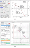 | Figure 1 Side-by-side Unified Fit of the same hierarchical aggregate dataset. (a) Irena (Igor Pro) Unified Fit panel and log–log graph; (b) pyIrena (Python) Unified Fit model dialog and graph. The two implementations reach essentially identical model parameters from independent code paths. |
5.2. Tiered analysis of bimodal nanoprecipitates in a metallic powder
Real-world SAS samples rarely have a single `best' analysis; the appropriate tool depends on how much physical detail the data can support, how much and what kind of information is needed for a specific scientific problem, and how much modeling effort the user is prepared to invest. Figs. 2–5 illustrate this point on a USAXS dataset from a metallic powder containing internal nanoprecipitates. The powder grains are themselves several micrometres across and therefore scatter well below the experimentally accessible Q range; in the measured window only the Porod tail of the grain-surface scattering is observed, manifested as a low-Q power law of slope −4. The signal of scientific interest is the additional scattering contributed by the internal nanoprecipitates, superimposed on this powder-grain Porod background. The chemical identity of the powder and its precipitates is not material to the present argument – the example is chosen to show how four Irena tools, of progressively greater physical sophistication, characterize the same dataset. While I use Irena tools here, the same analysis tools are also available in pyIrena and I could have used pyIrena for the same demonstration.
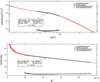 | Figure 2 Guinier fit returning a single Rg = 224 Å; the systematic standardized residual (lower trace) shows that one Gaussian-equivalent population is insufficient. |
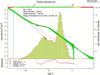 | Figure 3 MaxEnt size distribution (spheres) revealing a broad, apparently bimodal, volume distribution (diameter axis, as is conventional in the Irena Size Distribution panel). |
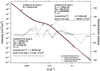 | Figure 4 Unified Fit uses two nanoprecipitate populations (Level 1 and Level 2) and a power-law level (Level 3) for the powder-grain surface scattering. Levels 1 and 2 each supply their own invariant, so the volume fractions of the two nanoprecipitate populations can be determined. For Level 3 the invariant, and hence the volume fraction, is not meaningful, because its Guinier component lies outside the measured Q range and cannot be included in the model. |
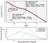 | Figure 5 Modeling tool fit using two explicit log-normal sphere distributions for the nanoprecipitates and one Unified level for the grain surfaces, returning parameterized size distributions and per-population volume fractions. |
Fig. 2 presents the simplest – and fastest – Guinier approximation analysis, which returns a single Rg = 224 Å, together with an I(0) from which a volume fraction may be estimated provided the scattering contrast is known and the data are on an absolute scale. The Guinier-region linear fit range (Qmin Rg ≃ 0.98 and Qmax Rg ≃ 2.16) was set visually and extends beyond the QRg < 1.3 range within which the Guinier approximation is normally applied; this, together with the standardized residual (lower trace) exhibiting clear systematic curvature, indicates that a single Gaussian-equivalent particle population is an inadequate description of the data. Yet, for quick comparison analysis among changing data, it may be fully sufficient.
Fig. 3 shows how inverting I(Q) with the MaxEnt size-distribution tool, assuming spherical scatterers, immediately reveals the cause of the residual structure: the recovered volume distribution is broad, with a range of particle diameters from 30 Å to over 1200 Å. Its mean and median diameters are 430 and 443 Å, its volume-weighted root-mean-square radius is 233 Å, and the shape of the size distribution suggests bimodality. For historical reasons the Size Distribution panel reports particle diameter, whereas other Irena tools use radius. To avoid this inconsistency, the pyIrena Size Distribution tool reports radius. The size-distribution analysis also returns the total of all scatterers when contrast and absolute scaling are known, but does not by itself decompose that total into per-population contributions. Inversion of I(Q) to a size distribution is an ill-posed problem whose solution depends on the assumed particle shape, the background, the regularization and the accessible Q range; under the assumptions used here, a is favored. The cumulative volume distribution reported alongside P(r) does, however, allow the volume fraction contained within any chosen size interval to be read off directly.
Fig. 4 shows Unified Fit with two levels assigned to the nanoprecipitate scattering and an additional level capturing the residual −4 slope from the powder-grain surfaces. A single-level Unified Fit description of the nanoprecipitate scattering was not satisfactory and left significant systematic residuals. This – and the bimodality revealed in Fig. 3 – motivates use of a higher number of Unified levels. Each level supplies its own invariant, so the volume fractions of the constituent populations are recovered independently of each other – a quantitative decomposition the Size Distribution tool, returning only a total cannot deliver. Obtaining a stable solution with two levels this close together is difficult and, depending on starting conditions, fitting results may not be stable and reproducible.
And finally, Fig. 5 shows analysis using the Modeling tool, which combines the per-population separation of the Unified Fit with the size-distribution detail of Fig. 3: each nanoprecipitate population is represented by an explicit log-normal distribution of spheres, while the powder-grain Porod tail is modeled as a single Unified level. The resulting fit returns, for each population, a parameterized distribution [mean, mode, median, full width at half-maximum (FWHM)] together with its own volume fraction. The two log-normal distributions are shown in the lower panel of Fig. 5 – population 2P with a volume-weighted root-mean-square radius of 270.8 Å (mean/mode/median/FWHM = 259.2/208.8/242.1/140.1 Å) and population 3P with a volume-weighted root-mean-square radius of 215.8 Å (mean/mode/median/FWHM = 197.8/142.8/179.1/155.6 Å); their separation is consistent with the bimodality independently revealed by the MaxEnt analysis. The Modeling tool allows the user to impose additional constraints that may be known from other types of characterization or theory – size-distribution type, form-factor shape, etc. – which grounds the results in materials expertise.
Because the four analyses report their results as different quantities – a radius of gyration in the Guinier and Unified Fit tools, a diameter in the Size Distribution panel, and the moments of a log-normal radius distribution in the Modeling tool – Table 2 places them on a common basis. Every method that resolves the dominant nanoprecipitate population places it at an equivalent sphere diameter of 400–520 Å, and the Guinier analysis, which necessarily returns a single I(0)-weighted average over the whole system, gives a larger apparent size, as expected. The Unified Fit additionally resolves a larger low-volume-fraction level near 900 Å that the size-distribution inversion does not separate from the rest of the distribution. The more demanding comparison is the total nanoprecipitate volume fraction, which depends on absolute intensity calibration and scattering contrast as well as on the fitted sizes: the three methods that determine it agree to within 15% – 0.043 (Size Distribution), 0.050 (Unified Fit) and 0.046 (Modeling).
| ||||||||||||||||||||||||||||||||||
Taken together, Figs. 2–5 illustrate a design choice of Irena and pyIrena: a single dataset can be analyzed at several levels of physical detail, each carrying a different cost–benefit balance. A single-parameter Guinier value is obtained in seconds and is appropriate where comparative ordering between samples suffices; a MaxEnt inversion exposes multimodality with minimal model commitment but does not separate populations quantitatively; a Unified Fit separates the populations and yields invariant-derived volume fractions for each, with relatively few model assumptions; and an explicit Modeling fit assigns a full parameterized size distribution to every population, allows the user to include additional knowledge in the model and recovers their population contributions to I(Q) by direct synthesis. Irena exposes all four routes from the same data record, allowing the analyst to escalate from screening through to publication-quality characterization without leaving the package. The system shown here is, by SAS standards, comparatively simple – only two populations of nominally spherical precipitates inside an inert powder; more complex systems with anisotropic scatterers, structure-factor effects, multi-phase aggregates or multiple contrasts extend the same hierarchy further still, drawing on the form-factor and structure-factor libraries summarized in Table 1 and detailed in the supporting information.
6. Availability, documentation and support
6.1. Irena
The main page is available from the Argonne USAXS website (https://usaxs.xray.aps.anl.gov/software-jan-ilavsky) and the source code is distributed via the GitHub SAXS_IgorCode repository (https://github.com/jilavsky/SAXS_IgorCode). The package is free to use (with US government copyright license). Irena 2.75 requires Igor Pro 9.04 or higher; Igor Pro is commercial software (WaveMetrics Inc.) for which a free 30-day trial is available from the vendor. The Irena Igor Pro source comprises ∼250 000 lines of Igor procedure code.
6.2. pyIrena
Source code is hosted at https://github.com/jilavsky/pyirena under the MIT license. Releases are published to the Python Package Index. The base install (pip install pyirena) provides the analytical core only; pip install pyirena[gui] adds the Qt graphical interface; pip install pyirena[mcp] adds the MCP server. The package pyIrena requires Python ≥ 3.10 and < 3.14, and runs on Linux, macOS and Windows. At the time of writing, pyIrena comprises ∼100000 lines of Python.
6.3. Documentation and user support
User support for both packages is provided by the author via email ([email protected]). An extensive manual is hosted at https://saxs-igorcodedocs.readthedocs.io. The pyIrena manual will be finalized when features of pyIrena stabilize. In the meantime, extensive AI-generated documentation including dedicated guides for the GUI quick-start, each analysis tool, the batch API, the NXcanSAS file layout and AI/MCP integration (docs/ai_integration.md, docs/ai_tools_reference.md) is available on GitHub (https://github.com/jilavsky/pyirena/tree/main/docs).
A YouTube channel at https://www.youtube.com/channel/UCDTzjGr3mAbRi3O4DJG7xHA provides instructional and educational movies. An Irena users mailing list is available on the APS mailman site (https://mailman.aps.anl.gov/mailman/listinfo/irena_users).
Bug reports can be submitted via email to the author or through the Irena GitHub issue tracker (https://github.com/jilavsky/SAXS_IgorCode/issues) or pyIrena GitHub issue tracker (https://github.com/jilavsky/pyirena/issues), as appropriate.
7. Community impact, validation and a note on AI-assisted development
The package pyIrena has been validated against Irena on a suite of synthetic datasets generated from exactly known parameters, so that both implementations are measured against a common ground truth rather than only against each other. The suite covers Size Distribution (MaxEnt inversion; sphere, spheroid and bimodal cases), Unified Fit (one and two levels), Modeling (a size-distribution population combined with a Unified level, with a diffraction peak, and with a hard-sphere structure factor), Simple Fits (six analytical models), WAXS (Gaussian and pseudo-Voigt) and the scattering-contrast calculator; starting parameters were offset from the truth, typically by a factor of 0.6, so that the tables demonstrate convergence rather than assume it. Over the 98 quantities both packages report, the median deviation from the known truth is 0.19% for pyIrena and 0.31% for Irena, and the median difference between the two packages is 0.04%; every pyIrena value lies within the tolerance enforced by its regression test suite. Only one row differs between the packages by more than 8%, and it reflects a difference in what is reported rather than in what was computed: pyIrena reports the diffraction-peak width as a Gaussian standard deviation and Irena reports it as a half-width at half-maximum, and converting between the two conventions recovers agreement to five significant figures. The remaining discrepancies above a percent or two are all weakly determined, strongly correlated quantities – most conspicuously the Unified power-law prefactor B, where in the two-level test both packages depart from the true value by the same +23% while agreeing with each other to 0.03%. Two independent implementations converging on the same value of an ill-determined parameter is a more informative result than either matching the truth would be. Because the reference values are exact by construction, this framework also validates the algorithms that pyIrena implements and Irena does not – the Monte Carlo size-distribution solver and the minority-phase topology metrics – which have no Irena counterpart to compare against; both are covered by the same regression tests. The complete tables, the settings used in each package and the generator that produced the data are given in Section S3 of the supporting information. Fig. 1 shows the corresponding comparison on experimental data. As a practical measure of the batch architecture, a two-level Unified Fit applied to 41 USAXS datasets on one MacBook Pro (M5 Max) takes ∼30 s using the Irena Scripting Tool and under 2 s using pyirena.batch – better than an order of magnitude faster. Both are wall-clock times for serial execution; the parallel execution path of pyirena.batch was not exercised in this comparison.
External validation is provided by 25 years of use across an exceptionally broad range of scientific fields. The original 2009 Irena publication (Ilavsky & Jemian, 2009) has been cited more than 2000 times. Highly cited studies making use of Irena span SAS methodology (Li et al., 2016), the characterization of natural porous media (Anovitz & Cole, 2015), the oriented nucleation of perovskite photovoltaic films (Shi et al., 2023) and the design of nanoporous carbon electrodes for sodium-ion batteries (Lan et al., 2025), among many others. This breadth – from energy materials and photovoltaics through geomaterials and biological systems – demonstrates that Irena's combination of GUI accessibility, hierarchical-model coverage and slit-smearing support has filled the gap it was designed to fill.
A second methodological observation deserves comment. The package pyIrena has been developed under a workflow in which the author plans the overall package structure, identifies features and the GUI, specifies the algorithm, validates numerical outputs against reference Irena results, and drives debugging; an LLM coding assistant performs the translation from the original Igor procedures – and the addition of new features – into the Python implementation. This division of labor is reflected in the pyIrena README byline (`Coded by Claude from SAXS_IgorCode Irena. Planned, defined, debugged, and validated by Jan Ilavsky.'). This model has allowed a single domain expert to deliver, in a few months, a Python port that covers the most heavily used Irena tools, adopts modern data standards (NXcanSAS/HDF5), introduces capabilities absent from the original (Monte Carlo size analysis, topology metrics, MCP integration), and is now installable on every major operating system. The same workflow can, in principle, be used to extend or modernize other long-lived domain-specific scientific software where the scarce resource is domain knowledge rather than coding effort.
8. Conclusions and outlook
Irena has, over 25 years, become a community resource for the analysis of SAS data from complex polydisperse hierarchical materials. Its development has been continuously driven by user requests, leading to a broad library of forward-modeling tools, size-distribution algorithms and supporting utilities. The package pyIrena now re-implements the most widely used of these tools in pure Python, removes the dependency on commercial software, adds bidirectional interoperability with Irena, and exposes the analyses through four coequal interfaces: a Qt graphical panel, a scriptable batch API, JSON replay and an MCP server for AI-agent access. Together, the two packages cover interactive GUI-driven analysis, headless high-throughput beamline pipelines and conversational LLM-driven exploration of data archives. The practical value of this arrangement is what Section 5.2 illustrates: a single data record can be escalated from a seconds-long Guinier screen to a fully parameterized multi-population model without leaving the package, and it is this workflow efficiency, rather than any individual algorithm, that I regard as the principal contribution of both packages.
Ongoing pyIrena development is focused on porting the remaining widely requested Irena-only tools, on extending the NXcanSAS write specification to cover all stored analysis metadata, on tighter integration with the new APS USAXS data-reduction pipeline and on expanding the MCP tool surface to cover write operations as well as the current read/analyze operations.
9. Related literature
The following references are only cited in the supporting information for this article: Allen et al. (1996), Ardell & Ozolins (2005), Beaucage (2004), Bevington & Robinson (2003), Debye & Bueche (1949), Huang et al. (2008), IUPAC (2021), Mulderig et al. (2017), Percus & Yevick (1958), Sears (1992), Sharma & Sharma (1977), Teixeira (1988), Teubner & Strey (1987), Thiele (1963), Wertheim (1963).
Supporting information
Supporting information. DOI: https://doi.org/10.1107/S1600576726009647/uu5035sup1.pdf
Acknowledgements
Over the past 25 years many colleagues contributed to Irena development by providing models, code, tools or suggestions, which helped guide the development. A short and incomplete list includes the late Greg Beaucage (Unified Fit), Peter R. Jemian (core early development, MaxEnt, regularization), Andrew Allen (fractal model), Andrew Nelson (reflectivity), Dale Schaefer (Unified Fit) and many others. The development was driven by the Irena user community, whose feedback and needs helped shape the package. Finally, the Anthropic Claude coding assistant for pyIrena translation has been critical. Anthropic Claude has also been used for drafting the various versions of this article from documentation, notes and manuscripts.
Conflict of interest
The author declares no conflict of interest.
Data availability
Irena with example data is available on GitHub (https://github.com/jilavsky/SAXS_IgorCode); pyIrena with example data is also hosted on GitHub (https://github.com/jilavsky/pyirena) (including pyIrena source code and documentation); documentation and tutorials are hosted at https://saxs-igorcodedocs.readthedocs.io (Irena documentation is available at https://saxs-igorcodedocs.readthedocs.io); finally, a YouTube channel with instructional movies is at https://www.youtube.com/channel/UCDTzjGr3mAbRi3O4DJG7xHA.
Funding information
This work was supported by the US Department of Energy, Office of Science, Basic Energy Sciences, under contract No. DE-AC02-06CH11357.
References
 Allen, A. J., Krueger, S., Skandan, G., Long, G. G., Hahn, H., Kerch, H. M., Parker, J. C. & Ali, M. N. (1996). J. Am. Ceram. Soc. 79, 1201–1212. CrossRef CAS Web of Science Google Scholar
Anovitz, L. M. & Cole, D. R. (2015). Rev. Mineral. Geochem. 80, 61–164. Web of Science CrossRef Google Scholar
Anthropic (2024). Introducing the Model Context Protocol, https://www.anthropic.com/news/model-context-protocol. Google Scholar
Ardell, A. J. & Ozolins, V. (2005). Nat. Mater. 4, 309–316. CrossRef PubMed CAS Google Scholar
Beaucage, G. (1995). J. Appl. Cryst. 28, 717–728. CrossRef CAS Web of Science IUCr Journals Google Scholar
Beaucage, G. (1996). J. Appl. Cryst. 29, 134–146. CrossRef CAS Web of Science IUCr Journals Google Scholar
Beaucage, G. (2004). Phys. Rev. E 70, 031401. CrossRef Google Scholar
Bevington, P. R. & Robinson, D. K. (2003). Data Reduction and Error Analysis for the Physical Sciences, 3rd ed. McGraw-Hill. Google Scholar
Bressler, I., Pauw, B. R. & Thünemann, A. F. (2015). J. Appl. Cryst. 48, 962–969. Web of Science CrossRef CAS IUCr Journals Google Scholar
Debye, P. & Bueche, A. M. (1949). J. Appl. Phys. 20, 518–525. CrossRef CAS Web of Science Google Scholar
Ding, L. & Do, C. (2026). J. Appl. Cryst. 59, 578–585. Web of Science CrossRef CAS IUCr Journals Google Scholar
Förster, S., Apostol, L. & Bras, W. (2010). J. Appl. Cryst. 43, 639–646. Web of Science CrossRef IUCr Journals Google Scholar
Franke, D., Gräwert, T. & Svergun, D. I. (2025). J. Appl. Cryst. 58, 1027–1033. Web of Science CrossRef CAS IUCr Journals Google Scholar
Franke, D., Jeffries, C. M. & Svergun, D. I. (2015). Nat. Methods 12, 419–422. CrossRef CAS PubMed Google Scholar
Hammouda, B. (2010). J. Appl. Cryst. 43, 716–719. Web of Science CrossRef CAS IUCr Journals Google Scholar
Hansen, P. C. (1998). Rank-Deficient and Discrete Ill-Posed Problems: Numerical Aspects of Linear Inversion. Philadelphia: Society for Industrial and Applied Mathematics. Google Scholar
Huang, E., Liaw, P. K., Porcar, L., Liu, Y., Liu, Y., Kai, J. & Chen, W. (2008). Appl. Phys. Lett. 93, 161904. Web of Science CrossRef Google Scholar
Ilavsky, J. & Jemian, P. R. (2009). J. Appl. Cryst. 42, 347–353. Web of Science CrossRef CAS IUCr Journals Google Scholar
Ilavsky, J., Jemian, P. R., Allen, A. J., Zhang, F., Levine, L. E. & Long, G. G. (2009). J. Appl. Cryst. 42, 469–479. Web of Science CrossRef CAS IUCr Journals Google Scholar
Ingham, B., Li, H., Allen, E. L. & Toney, M. F. (2011). J. Appl. Cryst. 44, 221–224. CrossRef CAS IUCr Journals Google Scholar
IUPAC (2021). Standard Atomic Weights. Commission on Isotopic Abundances and Atomic Weights, https://www.ciaaw.org/atomic-weights.htm. Google Scholar
Könnecke, M., Akeroyd, F. A., Bernstein, H. J., Brewster, A. S., Campbell, S. I., Clausen, B., Cottrell, S., Hoffmann, J. U., Jemian, P. R., Männicke, D., Osborn, R., Peterson, P. F., Richter, T., Suzuki, J., Watts, B., Wintersberger, E. & Wuttke, J. (2015). J. Appl. Cryst. 48, 301–305. Web of Science CrossRef IUCr Journals Google Scholar
Lake, J. A. (1967). Acta Cryst. 23, 191–194. CrossRef IUCr Journals Web of Science Google Scholar
Lan, N., Li, J., Zeng, L., Luo, D., Du, D., Li, X., He, H. & Zhang, C. (2025). Adv. Mater. 37, 2419528. CrossRef Google Scholar
Lawson, C. L. & Hanson, R. J. (1974). Solving Least Squares Problems. Englewood Cliffs: Prentice-Hall. Google Scholar
Li, T., Senesi, A. J. & Lee, B. (2016). Chem. Rev. 116, 11128–11180. Web of Science CrossRef CAS PubMed Google Scholar
Model Context Protocol Specification (2024–2026). Model Context Protocol, https://modelcontextprotocol.io. Google Scholar
Mulderig, A., Beaucage, G., Vogtt, K., Jiang, H. & Kuppa, V. (2017). J. Aerosol Sci. 109, 28–37. CrossRef CAS Google Scholar
NeXus International Advisory Committee (2020). NXcanSAS Application Definition, https://manual.nexusformat.org/classes/applications/NXcanSAS.html. Google Scholar
Parratt, L. G. (1954). Phys. Rev. 95, 359–369. CrossRef Web of Science Google Scholar
Percus, J. K. & Yevick, G. J. (1958). Phys. Rev. 110, 1–13. CrossRef CAS Web of Science Google Scholar
Petoukhov, M. V., Franke, D., Shkumatov, A. V., Tria, G., Kikhney, A. G., Gajda, M., Gorba, C., Mertens, H. D. T., Konarev, P. V. & Svergun, D. I. (2012). J. Appl. Cryst. 45, 342–350. Web of Science CrossRef CAS IUCr Journals Google Scholar
Petoukhov, M. V., Konarev, P. V., Kikhney, A. G. & Svergun, D. I. (2007). J. Appl. Cryst. 40, s223–s228. Web of Science CrossRef CAS IUCr Journals Google Scholar
Pospelov, G., Van Herck, W., Burle, J., Carmona Loaiza, J. M., Durniak, C., Fisher, J. M., Ganeva, M., Yurov, D. & Wuttke, J. (2020). J. Appl. Cryst. 53, 262–276. Web of Science CrossRef CAS IUCr Journals Google Scholar
Sears, V. F. (1992). Neutron News 3(3), 26–37. CrossRef Google Scholar
Sharma, R. V. & Sharma, K. C. (1977). Physica A 89, 213–218. CrossRef Google Scholar
Shi, P., Ding, Y., Ding, B., Xing, Q., Kodalle, T., Sutter-Fella, C. M., Yavuz, I., Yao, C., Fan, W., Xu, J., Tian, Y., Gu, D., Zhao, K., Tan, S., Zhang, X., Yao, L., Dyson, P. J., Slack, J. L., Yang, D., Xue, J., Nazeeruddin, M. K., Yang, Y. & Wang, R. (2023). Nature 620, 323–327. CrossRef CAS PubMed Google Scholar
Shrestha, S. et al. (2026). SasView, version 6.2.0, https://doi.org/10.5281/zenodo.20270235. Google Scholar
Skilling, J. & Bryan, R. K. (1984). Mon. Not. R. Astron. Soc. 211, 111–124. CrossRef Web of Science Google Scholar
Svergun, D. I., Semenyuk, A. V. & Feigin, L. A. (1988). Acta Cryst. A44, 244–250. CrossRef Web of Science IUCr Journals Google Scholar
Teixeira, J. (1988). J. Appl. Cryst. 21, 781–785. CrossRef Web of Science IUCr Journals Google Scholar
Teubner, M. & Strey, R. (1987). J. Chem. Phys. 87, 3195–3200. CrossRef CAS Web of Science Google Scholar
Thiele, E. (1963). J. Chem. Phys. 39, 474–479. CrossRef Google Scholar
Toby, B. H. & Von Dreele, R. B. (2013). J. Appl. Cryst. 46, 544–549. Web of Science CrossRef CAS IUCr Journals Google Scholar
Von Dreele, R. B. (2014). J. Appl. Cryst. 47, 1784–1789. Web of Science CrossRef CAS IUCr Journals Google Scholar
Wertheim, M. S. (1963). Phys. Rev. Lett. 10, 321–323. CrossRef Google Scholar
This is an open-access article distributed under the terms of the Creative Commons Attribution (CC-BY) Licence, which permits unrestricted use, distribution, and reproduction in any medium, provided the original authors and source are cited.
| JOURNAL OF APPLIED CRYSTALLOGRAPHY |