

 menu


computer programs
 | JOURNAL OF APPLIED CRYSTALLOGRAPHY |
 access
McSAS3: improved Monte Carlo small-angle scattering analysis software for dilute and dense scatterers

aBundesanstalt für Materialforschung und -Prüfung, Unter den Eichen 87, 12205 Berlin, Germany
*Correspondence e-mail: [email protected]
The Monte Carlo (MC) approach implemented in McSAS enables easy and flexible analysis of small-angle scattering (SAS) patterns, allowing the user to characterize the morphology of samples with a minimum of assumptions. The MC approach is able to fit most practical scattering patterns remarkably well (when reasonable uncertainty estimates are provided on the intensity), resulting in form-free model parameter distributions and distribution modes. Theoretically, these can be distributions on any model parameter, but in practice the MC-optimized parameter is usually a volume-weighted size distribution, in relative or absolute volume fraction for absolute-scaled data. McSAS3 is the refactored successor to the original McSAS Monte Carlo small-angle scattering analysis software. The refactored core now allows for use of the extensive `SasModels' form- and structure-factor library, is easy to integrate in fully automated data processing pipelines, but still remains well suited to process individual (batches of) scattering data. McSAS3 now also comes with a graphical user interface, McSAS3GUI, complete with guides, examples and videos. McSAS3GUI will aid in generating and testing the three configuration files needed for the McSAS3 core. These configuration files specify the data read-in, MC optimization and histogramming. The user interface can also be used to process individual files or batches (of over 1000 files if needed), and can be augmented with instrument-specific templates for easier use at specific beamlines and in laboratories.
Keywords: small-angle scattering; data analysis; Monte Carlo; size distributions; software; McSAS3.
1. Introduction
Assuming a proper automated data correction pipeline is in place (cf. Pauw et al., 2017 ), data analysis is often the most time consuming step in a small-angle scattering experiment. With classical least-squares analysis, e.g. using SasView (Shrestha et al., 2026b) or SASfit (Kohlbrecher & Breßler, 2022), time is needed to create a sample-appropriate model. This model typically consists of a scatterer model, parameter distribution form and inter-structure scattering descriptions. This triad then needs adapting and augmentation so it is able to match the peculiarities of real-life morphologies and measurements [a good example of which is shown by Henning et al. (2022)]. This becomes much more complex in dynamic experiments where the structure may evolve beyond the model during the experiment.
The Monte Carlo (MC) method offers a significant advantage here, in that the parameter distribution form no longer needs to be specified (Pauw et al., 2013b). Only the overall scatterer morphology (`form factor') and optionally the inter-particle scattering (`structure factor') now need to be defined. As fewer choices means less chance for human bias in the result (Pauw et al., 2023), reproducibility is improved. Once the form factor and optional structure factor are configured in accordance with the overall sample morphology, the optimization can start.
The MC procedure will then attempt to match the measured data ( ) with the MC data (
 ) (Pauw et al., 2013b). This comprises an inverse volume-weighted sum of independent, individual model contributions
Ik. The optimization is performed by randomly varying a specific parameter of the
 individual model contributions within predefined limits, and selecting the new parameter value when the match improves. The resulting parameter distributions are often less `smooth' as compared with the parametrized distribution shapes of the classical models (such as normal, log-normal or Schultz distributions), but can more closely describe the reality of the structure in a greater range of samples.
Over the past decade, the original McSAS (Bressler et al., 2015) has seen widespread use, with its accompanying paper having been cited over 200 times already. One of the first examples demonstrating its utility was to describe the complex size distribution evolution during the synthesis of quantum dots, which allowed the reaction mechanism to be identified (Abécassis et al., 2015). Other applications of the software include studying defect formation in titanium alloys (Wu et al., 2025), condensed phases in magnetic fluids (Mamiya et al., 2021), nanoparticles synthesized by laser ablation (Letzel et al., 2017), liquid metal droplets in composites (Crater et al., 2022) and pores in energy storage materials (Qiu et al., 2025). The vast majority use McSAS as a convenient tool for minimal-assumption nanostructural sizing, usually in combination with other methods such as electron microscopy for comparability and scatterer shape verification.
However, the original McSAS had issues that were impossible to resolve without a major rewrite. For example, the graphical user interface (GUI) was inseparable from the core, preventing headless operation or integration in automated data processing pipelines. Secondly, the number of supported models was rather limited, and it did not support multicore processing. Most frustratingly from a usage perspective, it was not possible to change the histogram settings without having to redo the complete (and occasionally time-consuming) optimization. Therefore, McSAS3 was made as a complete rewrite of the original code. While software is never truly finished, McSAS3 + GUI, shown in Fig. 2, now exceeds the `good enough' state where it is usable by the wider public. So far, McSAS3 has been used (amongst others) on large quantities of data from operando electrochemistry experiments (Jansske et al., 2025) and a wide range of data from different distributions of metal–organic framework samples (Smales et al., 2025). It has furthermore already been used to characterize mesostructured cellular foams (Morales-delaRosa et al., 2025), titanium alloys (Brumbauer et al., 2025), cellulose (Zhong et al., 2026), cellulose-derived hard carbons (Scheer et al., 2026), keratin fibers (Czibula et al., 2026) and porous polymers (Bilican et al., 2026).
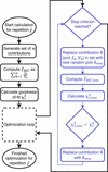
Briefly summarizing the original McSAS papers, the underlying working principle behind this implementation is as follows and shown schematically in Fig. 1. A set of scattering contributions is generated with (at least) one parameter randomly picked within configured limits, and scaled with the inverse of their volume [so as to most efficiently and most closely represent the information content in a scattering pattern (cf. Pauw et al., 2013b)]. The intensity comprising the sum of these contributions is compared with the measured intensity after a rapid least-squares optimization of a scale factor and background, relying on uncertainty estimates on the measurement to inform the precision of the measured data. A cyclic optimization is then started, where a single contribution in the set is replaced with another randomly generated contribution, and the new resulting sum compared with the measured data. An improvement in agreement between the model and measured data leads to an acceptance of the replacement, a degradation in agreement will lead to a rejection of the replacement. This process is repeated either until the match between model and measurement described through the goodness-of-fit `convergence criterion' is reached or until the configured maximum number of iterations or accepted steps is reached. This entire optimization is repeated a number of times (`number of repetitions') with new random number generator seeds, so that a number of independent solutions are generated.
|
Figure 1
A simplified representation of the optimization strategy used in McSAS and McSAS3, with the core optimization shown in blue. Multiple independent optimizations can be run in parallel in McSAS3, but sequentially in the original McSAS. |
The optimized parameter(s) are then converted to volume fractions through calculation of the volume of each contribution in the set, combined with the scaling information from the last least-squares optimization. If the data are supplied in absolute units, and if the X-ray scattering contrast has been correctly set in the optimization configuration, the resulting volumes are absolute volume fractions of that contribution in the whole. Through histogramming of these volumes into bins, a size histogram (strictly distinct from a size distribution, which is its non-integrated sibling) is obtained, expressed in relative, or conditionally in absolute volume fraction. Uncertainties on the resulting size histogram are obtained through determination of the standard deviation of the histogramming results of the independent repetitions. These uncertainties thus provide some insight into the strength of the evidence for that particular histogram bin (cf. Bressler et al., 2015). A key point in the McSAS optimization is that the result reflects a volume-weighted size histogram. While this can be numerically converted to a number-weighted distribution, this practice is discouraged as it leads to small-sized contributions dominating the size histogram with concomitantly large uncertainties, obscuring the practically relevant, less numerous but larger contributions that are responsible for the majority of scattering in the measurement.
For more detail on the underlying optimization principles as well as a good number of examples, we refer readers to the older literature on its predecessor (Pauw et al., 2013b; Bressler et al., 2015). In this work, we will highlight the improvements that McSAS3 + GUI (Fig. 2) bring compared with the original. Some of the improvements will be demonstrated by three practical examples.
|
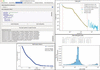
Figure 2
The panels of the McSAS3GUI user interface showing an optimization on a ZIF-8 dataset, with the main GUI shown in the top left, the loaded, clipped, rebinned data and fit shown in the top right, the output PDF in the bottom left with the data and size distribution, and the evolution of the optimization parameter in the bottom right. |
2. Advantages of McSAS3 compared with the original McSAS
McSAS3 offers the following advantages over the original (see Table 1):
|
||||||||||||||||||||||||||||||||

(i) The McSAS3 core is designed to be integrated in automated data workflows, and can be executed from the command line or a Jupyter notebook using configuration files. This scriptability allows for immediate, in-line analysis of data during an experiment as well.
(ii) Input data are supported from either ASCII or HDF5 containers. Data read-in options can be specified in detail using a YAML configuration file, to adapt to a wide range of variants such as CSV, NeXus, NeXish (looks like NeXus but does not quite conform to the standard; this is implemented at most synchrotron beamlines as well as our MOUSE instrument) and Anton Paar's (now superseded) `PDH' format.
(iii) The data read-in supports specifying input units for the scattering vector (Q) and scattering cross section (I) of the input data. These will be automatically converted to 1/nm and 1/(m sr). Fit-parameter size units will be in nm, the static units are in SasModels units (see SasModels documentation; Kienzle et al., 2025; Shrestha et al., 2026a). It is hoped that this feature may partially address the ostensibly pervasive unit scaling issues in small-angle X-ray scattering (SAXS) data analysis, as brought to light by the Data Analysis Round Robin experiment (Pauw et al., 2023).
(iv) The main models library is SasModels (Kienzle et al., 2025; Shrestha et al., 2026a) from the SasView (Shrestha et al., 2026b) community. This means that many (compiled) models are supported, and can be used in combination with some structure factors. The only limitation is that the chosen form factor model must specify a volume. Combinations of models can even be constructed using a simple syntax (e.g. `sphere@hardsphere+cylinder'), although it is recommended to keep models as simple as possible to avoid ambiguous results.
(v) There is a possibility to use simulated data as a model, as demonstrated in Section 4.3. This can be helpful for scatterer morphologies that are unsupported by SasModels. This also makes it possible to use any reference data of a monodisperse scatterer as a basis (e.g. a protein building block), and determine the size dispersity and/or aggregation number of that scatterer in the sample.
(vi) Multi-threaded processing is implemented for the independent repetitions, making sure modern computers can now be used as a space heater again. Each process writes its intermediate results directly to the output HDF5 container.
(vii) The user can now re-histogram any completed optimization to their heart's desire, without having to redo the optimization.
(viii) McSAS3 was built in a very modular fashion, making it easy to maintain, upgrade and extend.
While these are all, in principle, features of the McSAS3 core, we have recently also developed a separate PyQT6-based graphical user interface (McSAS3GUI) that can help adoption by lowering the barrier to the use of McSAS3. The user interface helps with the generation of the three configuration files needed for the core (one for data read-in, one for the model and optimization settings, and one for the histogramming settings), and has tabs to execute batch fitting and batch histogramming. Furthermore, it has a user guide with templated examples, that can be extended to include user-specific templates for projects or bespoke configurations for beamlines and laboratory instruments. Video guides are also available that explain the underlying principles, and demonstrate the use of McSAS3 with some general tips and tricks.
3. Administrative details
The code and issue lists are available on Github for the core (Pauw & Bressler, 2025a) and for the GUI separately (Pauw & Bressler, 2025b). By using `pip install McSAS3GUI' in an appropriate Python environment, the core McSAS3 is installed automatically as a dependency. The code is in active development and will be supported for at least several years, resources permitting. The core and GUI are released under an MIT license. A CI/CD pipeline has been implemented with an extensive test suite and experimental standalone binary builds, and contributions are very welcome using pull requests.
4. Use examples
4.1. Use example 1: Data Analysis Round Robin bimodal gold nanoparticle suspension
The first example shows how McSAS3 can be used to determine the modality of distributions, using data from the small-angle scattering Data Analysis Round Robin experiment (Pauw et al., 2023). This was an experiment to find out how the results of a small-angle scattering analysis may depend on the person who is carrying out the analysis. To this end, we collated four datasets of dispersions of spherical scatterers, and provided: the four three-column text files with the data; a document with information on the units, the sample composition and photon energy used for the collection of the data; an Excel sheet in which the researcher could fill in their results.
The results of this were published by Pauw et al. (2023), and the original information and datasets sent out to participants were published by Pauw & Smales (2023). This example uses the first dataset, which is a measurement of a bimodal gold nanoparticle suspension. The smaller population was half the size and only 10% in quantity of the larger population, to ensure the signal of the smaller particles is sufficiently hidden.
This dataset is included as an example in McSAS3, which can fit this dataset with minimal effort.1 The ten independent optimizations of this example are completed in 4 s on a MacBook Pro M1, with the histogramming taking about a second more.
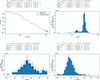
The resulting histogram (Fig. 3) shows the data and the fit in the leftmost panel, then the overall radius distribution, then just the small population, and lastly the large population. Population statistics showing the total volume fraction and volume-weighted population parameters (mean, variance, skew and kurtosis) of each individual range are shown above the individual histograms. It is recommended to express the population distribution width as a standard deviation by taking the square root of the variance.
|
Figure 3
The analysis result of scattering from a bimodal gold nanoparticle suspension. Top left: data and fit. Top right: overall size histogram. Bottom left: first population. Bottom right: second population. Note that the lower graphs use linear binning edges, and therefore show a slightly different histogram than when using logarithmically spaced histogram bin edges (as used in the top-right figure). |
4.2. Use example 2: Data Analysis Round Robin bimodal silica powder
The second example demonstrates the use of McSAS3 on powder samples. It uses the third dataset of the aforementioned Data Analysis Round Robin, which contains a measurement of a powder mixture of two vastly different sizes of spherical silica particles. As this is an intercalating powder of low-polydispersity particles, there is a significant structure factor present. We include the structure factor in the model by using the SasModels `hard-sphere' structure factor with Percus–Yevick closure (Percus & Yevick, 1958) and a local monodisperse approximation to use this monodisperse structure factor in a polydisperse system. (Due to the design of the optimizer engine, each contribution is unaware of the total population. Therefore, structure-factor approximations that use the full size distribution cannot be used in this MC approach.)
For data like this example, if there are significant structure factors and large structure scattering, we want to increase the maximum dimension in the model size parameter to ensure we can easily get an  Porod slope from the smallest Q (alternatively, the McSAS3 run configuration now also optionally fits a Porod slope as a background contribution). Secondly, we also need to limit the data range in the data read-in configuration to avoid the wide-angle silica scattering hump. Furthermore, we increase the number of contributions to reduce the granularity of the resulting parameter distributions at the cost of increased computation time.
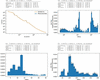
This sample is a bit more challenging to analyze than Example 1, but with the right settings we arrive at valid solutions (such as shown in Fig. 4). Note how the size distribution is affected by the configured volume fraction; valid answers can be obtained with a structure-factor volume fraction parameter ranging from ∼0.46 to 0.6. This highlights that it is not possible to get both volume fraction and size distribution uniquely, but that the user must fix one to retrieve the other as they are inextricably linked. To obtain the result in Fig. 4, we chose 0.55 because of speed: it is one of the fastest settings. The overall resulting distribution as well as the two isolated populations can be seen in Fig. 4.
|
Figure 4
The analysis result of scattering from a dense, bimodal silica powder. Top left: data and fit. Top right: overall size histogram. Lower left: first population. Lower right: second population. |
4.3. Use example 3: using a custom simulated form factor on a dispersion of faceted cubes
The third example demonstrates how McSAS3 can be used for shapes without analytical scattering functions. For these cases, simulated scattering patterns can be used as a basis model.
The European Metrology Programme for Innovation and Research (EMPIR) `nPSize' project set out to make non-spherical reference materials. These narrow-dispersity, faceted cubes are sample number 4 from that project. As no analytical models for faceted cubes exist, the analysis with McSAS3 can be done using a model interpolated from a single scattering simulation of a faceted cube (Deumer et al., 2022). The resulting parameter distribution will then be the (uniform) scaling factors for this model object.
Measurements of these nanoparticles were performed at the SAXS beamline at the Physikalisch-Technische Bundesanstalt (PTB). The data are publicly available from Zenodo (Deumer & Gollwitzer, 2022). The form factor model is a special `sim' type, which requires the simulated arrays for Q, I and  of the form factor data to be specified in the model description. This model should be complete, and include a (flat) Guinier region at the start, and Porod region at the end. Parameters for extrapolation beyond the data are then determined automatically.
The faceted cube data were simulated using the SPONGE, a software tool for simulating scattering from complex structures using the Debye equation, also described by Deumer et al. (2022). The model was an STL file of a faceted cube with a face-to-face distance of 1 nm. This means the scaling factors in the final histogram are identical to the object size distribution in nm.
The result from the McSAS3 optimization using this form factor is the set of scaling factors of the objects that, as an ensemble, best fit the data. This `sim' model fit assumes that a uniform scaling of the object results in a volume-squared intensity scaling and an inverse Q-axis scaling. The `sim' model can work in absolute units if the form factor model data themselves are supplied in absolute units.
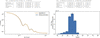
Due to the very small data uncertainties, scaling factor range and/or discrepancies between model and reality, a full convergence to a reduced chi-squared of 1 cannot be obtained but can be approached. The result is shown in Fig. 5.
|
Figure 5
The analysis result of scattering from a suspension of faceted cubes. Left: data and fit, right: isolated population showing the size distribution of faceted cubes. |
5. Adapting McSAS3 for laboratory and synchrotron data pipelines
Given the increased quantities of data from both synchrotron beamlines and laboratory sources, the burden of data analysis on scientists becomes even more pressing. Simultaneously, there is a trend towards more in situ and operando experiments even in the laboratory. Some researchers also aim to integrate X-ray scattering as a part of autonomous material optimization feedback cycles. (Despite the nomenclature, in real life these automated set-ups actually require a large investment in highly skilled personnel for the continuous integration, programming and operation.) These trends strongly benefit from integrated, flexible data pipelines with analyses, if for nothing else than to gain an initial insight into the trends and developments. McSAS3 has been written largely for this purpose.
To encourage use of the software, the instrument responsible can make the data read-in configurations available for their instrument or data source. Likewise, a small library of optimization templates can be prepared which optimize with simple, near-universal models (spheres being the most practical example, either with a structure factor for powders or without for most other samples). These should be configured so that the optimizer completion criteria are mostly limited by (i) the maximum number of accepted moves, and (ii) the maximum number of attempts, in order to keep the running time reasonable. It is worth remembering here that the success of the optimizer is strongly dependent on reasonable uncertainty estimates on the data, and so a thorough data correction pipeline is essential (Pauw et al., 2017).
Once this is in place, this quick run of McSAS3 can be attached to the data processing pipeline, to provide users with (near-)immediate insight into their material development and to provide morphological data for feedback cycles and material optimizers to work with. Based on the results from the McSAS3 optimizations, a more artisanal analysis can be developed if required.
6. Current limitations
Software is never feature-complete, and McSAS3 is no different. There are two limitations to bear in mind for now:
(i) Anisotropic data are supported in principle. The underlying fitting engine McSAS3 can take isotropic 1D or anisotropic 2D data and fit either [a very early example of this concept is demonstrated by Pauw et al. (2013a), and a test case for 2D anisotropic data fitting is included in the McSAS3 test suite]. The limiting factor for fitting anisotropic 2D data at the moment is the lack of 2D visualization support for data and results in McSAS3GUI. Such visualizations can be implemented if a common use case surfaces that is worth the effort.
(ii) There is no currently no good mechanism in place to interrupt a single optimization, and if settings are poorly chosen, it can run for a very long time. Pressing `abort' at the moment will only prevent further repetitions from being run, rather than abort the currently running (parallel) optimization processes. For now, the recommendation is to start doing (test) optimizations only after carefully selecting appropriate settings for the maximum number of iterations.
7. Conclusions
The hard limitations imposed by the original implementation of McSAS have now been resolved through a complete rewrite in McSAS3. McSAS3 is intended to be integrated as part of an automated data processing pipeline, and the additional McSAS3GUI provides an easy interface both for configuring the McSAS3 core and for fitting smaller batches of data (e.g. several thousands of data files). The examples demonstrate the broad utility of the approach and implementation, as shown for bimodal particle dispersions, bimodal powders and dispersions of scatterers with uncommon shapes. While the software will steadily improve in the future, the current state will undoubtedly be useful to many.
Footnotes
1After starting McSAS3GUI, select the `round_robin_dataset_1.yaml' example/template, go to the `McSAS3 Optimization…' tab, click the `Run McSAS3 Optimization…' button, then go to the `Histogram Settings' tab and click `Test Histogramming'. As this is just one file, this test will generate the one PDF file and open it. The `(Re-)Histogramming…' tab will do the same, but not open the PDF file, and is intended more for histogramming batches of files.
Acknowledgements
The text of this manuscript was written by the authors without the use of large language models. Parts of the code were implemented with the assistance of OpenAI Codex and were reviewed and tested by the authors. We are aware that tools of this kind are built on knowledge and code contributed by people who were never asked, and who cannot be credited individually here. We thank them nonetheless. Open access funding enabled and organized by Projekt DEAL.
References
 Abécassis, B., Bouet, C., Garnero, C., Constantin, D., Lequeux, N., Ithurria, S., Dubertret, B., Pauw, B. R. & Pontoni, D. (2015). Nano Lett. 15, 2620–2626.
Web of Science
PubMed
Google Scholar
Bilican, A., Sharma, P., Smales, G. J., Leutzsch, M., Farès, C., Ehmann, H., Moser, A., Weidenthaler, C. & Schmidt, W. (2026). Small Sci. 6, e202500460.
CrossRef
PubMed
Google Scholar
Bressler, I., Pauw, B. R. & Thünemann, A. F. (2015). J. Appl. Cryst. 48, 962–969.
Web of Science
CrossRef
CAS
IUCr Journals
Google Scholar
Brumbauer, F., Okamoto, N. L., Materna, P., Smales, G. J., Ichitsubo, T., Sprengel, W. & Luckabauer, M. (2025). Mater. Des. 259, 114711.
CrossRef
Google Scholar
Crater, E. R., Tutika, R., Moore, R. B. & Bartlett, M. D. (2022). Soft Matter 18, 7762–7772.
CrossRef
CAS
PubMed
Google Scholar
Czibula, C., Schaubeder, J. B., Smales, G. J., Chatterjee, J. B., Fisher, N. C., Silverstein, D. S., Thoman, M., Ghezzi, K. T., Richards, J. J. & Chazot, C. A. C. (2026). ACS Mater. Au 6, 163–176.
CrossRef
CAS
PubMed
Google Scholar
Deumer, J. & Gollwitzer, C. (2022). npsize_saxs_data_ptb, https://doi.org/10.5281/zenodo.5886834.
Google Scholar
Deumer, J., Pauw, B. R., Marguet, S., Skroblin, D., Taché, O., Krumrey, M. & Gollwitzer, C. (2022). J. Appl. Cryst. 55, 993–1001.
CrossRef
CAS
IUCr Journals
Google Scholar
Henning, L. M., Müller, J. T., Smales, G. J., Pauw, B. R., Schmidt, J., Bekheet, M. F., Gurlo, A. & Simon, U. (2022). Nanoscale Adv. 4, 3892–3908.
CrossRef
CAS
PubMed
Google Scholar
Jansske, K., Alvarez Ferrero, G. et al. (2025). In preparation.
Google Scholar
Kienzle et al. (2025). SasModels v.1.0.12, https://github.com/SasView/sasmodels.
Google Scholar
Kohlbrecher, J. & Breßler, I. (2022). J. Appl. Cryst. 55, 1677–1688.
Web of Science
CrossRef
IUCr Journals
Google Scholar
Letzel, A., Gökce, B., Wagener, P., Ibrahimkutty, S., Menzel, A., Plech, A. & Barcikowski, S. (2017). J. Phys. Chem. C 121, 5356–5365.
CrossRef
CAS
Google Scholar
Mamiya, H., Sudo, H., Cuya Huaman, J. L., Suzuki, K., Miyamura, H. & Balachandran, J. (2021). J. Phys. Chem. C 125, 740–748.
CrossRef
CAS
Google Scholar
Morales-delaRosa, S., Smales, G. J., Martínez-Triguero, J. & Melián-Cabrera, I. (2025). Microporous Mesoporous Mater. 381, 113322.
Google Scholar
Pauw, B. R. & Bressler, I. (2025a). McSAS3, https://github.com/BAMresearch/McSAS3.
Google Scholar
Pauw, B. R. & Bressler, I. (2025b). McSAS3GUI, https://github.com/BAMresearch/McSAS3GUI.
Google Scholar
Pauw, B. R., Ohnuma, M., Sakurai, K. & Klop, E. A. (2013a). arXiv, 1303.2903.
Google Scholar
Pauw, B. R., Pedersen, J. S., Tardif, S., Takata, M. & Iversen, B. B. (2013b). J. Appl. Cryst. 46, 365–371.
CrossRef
CAS
IUCr Journals
Google Scholar
Pauw, B. R. & Smales, G. J. (2023). Small-Angle Scattering Data Analysis Round Robin: Original for Participants, https://doi.org/10.5281/zenodo.7506365.
Google Scholar
Pauw, B. R., Smales, G. J., Anker, A. S., Annadurai, V., Balazs, D. M., Bienert, R., Bouwman, W. G., Breßler, I., Breternitz, J., Brok, E. S., Bryant, G., Clulow, A. J., Crater, E. R., De Geuser, F., Del Giudice, A., Deumer, J., Disch, S., Dutt, S., Frank, K., Fratini, E., Garcia, P. R. A. F., Gilbert, E. P., Hahn, M. B., Hallett, J., Hohenschutz, M., Hollamby, M., Huband, S., Ilavsky, J., Jochum, J. K., Juelsholt, M., Mansel, B. W., Penttilä, P., Pittkowski, R. K., Portale, G., Pozzo, L. D., Rochels, L., Rosalie, J. M., Saloga, P. E. J., Seibt, S., Smith, A. J., Smith, G. N., Spiering, G. A., Stawski, T. M., Taché, O., Thünemann, A. F., Toth, K., Whitten, A. E. & Wuttke, J. (2023). J. Appl. Cryst. 56, 1618–1629.
Web of Science
CrossRef
CAS
IUCr Journals
Google Scholar
Pauw, B. R., Smith, A. J., Snow, T., Terrill, N. J. & Thünemann, A. F. (2017). J. Appl. Cryst. 50, 1800–1811.
Web of Science
CrossRef
CAS
IUCr Journals
Google Scholar
Percus, J. K. & Yevick, G. J. (1958). Phys. Rev. 110, 1–13.
CrossRef
CAS
Web of Science
Google Scholar
Qiu, C., Wu, Y., Mai, X., Zhang, J., Guo, L., Zhao, Y., Zhu, Y., Lin, Z., Qiu, D., Li, A., Chen, X., Yang, H. Y. & Song, H. (2025). Small Methods 9, e01078.
CrossRef
PubMed
Google Scholar
Scheer, A., Tran Nguyen, H. B., Fischer, J., Smales, G. J., Selinger, J., Alem, A., Bandl, C., Fischer, S., Mikhailova, D. & Spirk, S. (2026). Carbon 260, 121941.
CrossRef
Google Scholar
Shrestha, S. et al. (2026a). SasModels v.1.0.12: Theory Models for Small Angle Scattering, https://dx.doi.org/10.5281/zenodo.20270238.
Google Scholar
Shrestha, S. et al. (2026b). SasView for Small Angle Scattering Analysis, https://dx.doi.org/10.5281/zenodo.20270235.
Google Scholar
Smales, G. J., Appel, P. A., Breßler, I., Chambers, A., Dumele, O., Ebisch, M., Frontzek, J., del Refugio Monroy, J., Rosalie, J. M. & Pauw, B. R. (2025). ChemRxiv, https://publcif.iucr.org/journals/misc/refs.html.
Google Scholar
Wu, Z., Shi, Y., Yang, Q., Song, Z., Wang, Q., Ma, R., Zhang, P., Chen, Y., Li, Z., Yu, R., Zhu, T., Wan, M. & Cao, X. (2025). Vacuum, 240, 114526.
Google Scholar
Zhong, C., Ubiparip, Z., Galicia-Andrés, E., Smales, G. J., Oostenbrink, C., Desmet, T. & Nidetzky, B. (2026). ACS Catal. 16, 13007–13021.
CrossRef
CAS
Google Scholar
This is an open-access article distributed under the terms of the Creative Commons Attribution (CC-BY) Licence, which permits unrestricted use, distribution, and reproduction in any medium, provided the original authors and source are cited.
| JOURNAL OF APPLIED CRYSTALLOGRAPHY |