Learning lattice parameters from powder X-ray diffraction data using invariants

Hofgard, E.; Min, K.; Segal, N.; Mittan-Moreau, D.W.; Tehrani, A.M.; Oklejas, V.; Gómez-Bombarelli, R.; Nigam, J.; Paley, D.W.; Brewster, A.S.; Smidt, T.

doi:10.1107/S2053273326010284

research papers

FOUNDATIONS
ADVANCES

ISSN: 2053-2733

Volume 83| Part 1| January 2027|

https://doi.org/10.1107/S2053273326010284

Open

access

Learning lattice parameters from powder X-ray diffraction data using invariants

^aMassachusetts Institute of Technology, Cambridge, MA, USA, and ^bMolecular Biophysics and Integrated Bioimaging Division, Lawrence Berkeley National Laboratory, Berkeley, CA, USA
^*Correspondence e-mail: [email protected]

Edited by A. Singer, Princeton University, USA (Received 1 July 2026; accepted 5 October 2026)

We present a machine learning (ML) method to determine unit-cell parameters from powder X-ray diffraction (XRD) data using a novel invariant lattice representation. In ML, the data representation used can have a substantial impact on the prediction quality. Previous approaches have directly predicted lattice parameters (a, b, c, α, β, γ) from XRD inputs. However, these parameters depend strongly on the unit-cell reduction or convention used. In this work, we construct an invariant representation of the reciprocal lattice that is independent of primitive-cell convention, based on the bispectrum – a descriptor built from spherical harmonic projections of lattice points. The calculation of the lattice bispectrum is differentiable, and we demonstrate how to invert it using gradient-based optimization initialized from a nearest-neighbor lookup. We show that, with a fixed ML model architecture, using the lattice bispectrum as the ML target rather than the unit-cell parameters leads to more accurate lattice parameter predictions. For example, using the MP-20 dataset, a subset of the Materials Project database, the bispectrum reduces length mean absolute percentage error (MAPE) from 11.08% to 2.43% and angle MAPE from 12.15% to 2.45% compared with direct prediction with the same model architecture. We additionally benchmark our approach against pre-existing XRD data to crystal structure models such as Crystalyze and assess its performance on experimental data. Beyond unit-cell representation, we anticipate this invariant lattice representation could serve more broadly as a geometry-aware target for other crystallographic ML tasks such as structure generation.

Keywords: powder diffraction; machine learning; artificial intelligence; lattice parameter determination; representation learning.

1. Introduction

Powder X-ray diffraction (XRD) is a core tool for characterizing materials. In general, traditional methods extract peak positions and then assess trial unit cells in order to determine the correct lattice parameters. With the advent of machine learning (ML), interest has grown in using ML to aid in unit-cell determination. ML models are able to learn patterns in large-scale datasets and thus could be used in conjunction with crystallographic expertise to narrow the lattice parameter search space (Chitturi et al., 2021 ; Dong et al., 2021 ; Habershon et al., 2004 ). However, even setting aside challenges in signal quality such as peak overlap (David & Shankland, 2008 ), ML approaches face a fundamental representation challenge, as the unit cell is not a unique representation for a given lattice. Small distortions can change the reduced-cell convention discontinuously, creating an inherently non-smooth learning target. Previous ML approaches for learning lattice parameters from XRD data have usually directly predicted the lattice parameters ( $[a,b,c,\alpha,\beta,\gamma]$ ) which depend on the unit-cell convention used.

Throughout this work, we refer to cubic, hexagonal and tetragonal systems as high-symmetry, as their lattice parameters are the most constrained. Low-symmetry triclinic and monoclinic systems are challenging due to having the greatest number of free lattice parameters. Previous work has struggled to obtain accurate predictions for low-symmetry crystal systems, as the parameter space is larger and multiple reduced-cell conventions can represent the same lattice (Chitturi et al., 2021; Andrejevic et al., 2026 ; Shu et al., 2025 ; Gómez-Peralta et al., 2023 ; Gómez-Peralta et al., 2025 ). We address this by introducing an invariant lattice representation in reciprocal space that is independent of primitive-cell convention, based on the bispectrum (Bartók et al., 2013 ). The lattice bispectrum is constructed from spherical harmonic projections of lattice points in reciprocal space and varies smoothly under continuous lattice deformations, providing a more learnable target for a neural network. We demonstrate that this representation can be inverted in an auto-differentiable framework.

While many previous ML works use convolutional neural networks (CNNs) (Chitturi et al., 2021; Gómez-Peralta et al., 2023), these models lose information in long-range XRD peak dependencies. By the construction of their architecture, CNNs are translation invariant. This means that, while a CNN may detect individual peaks, it cannot directly relate peaks across the full diffraction pattern. This is a useful inductive bias for images, yet it does not align with our understanding of XRD data. Peak positions carry absolute physical meaning and cannot be treated as interchangeable regardless of their location. In contrast, self-attention mechanisms in transformers compute pairwise interactions between all positions simultaneously, allowing every peak to attend to every other peak across the full diffraction pattern in a single layer.

We thus train a transformer to predict the lattice bispectrum from XRD data and compare performance with directly predicting the lattice parameters. The model takes as input a simulated or experimental XRD pattern and outputs the lattice bispectrum, from which lattice parameters are recovered via inversion, leading to more accurate predictions than directly predicting lattice parameters. See Fig. 1 for our proposed workflow. We train our model using simulated XRD patterns from the Materials Project (Jain et al., 2013 ; Horton et al., 2025 ) with physically informed data augmentation. We benchmark model performance on experimental XRD patterns in the RRUFF database (Lafuente et al., 2015 ) and on unit cells with dominant zones. To summarize, our main contributions are:

Figure 1
Workflow for predicting the bispectrum and then inverting to obtain lattice parameters. The model is given an input XRD pattern represented as an array of (2θ, intensity) values and is trained to predict the lattice bispectrum. The prediction can then be inverted to obtain a set of spanning lattice vectors (see Section 4.2

). Postprocessing using cctbx or pymatgen can then be done to obtain lattice parameters in a standardized or conventional setting.

(i) We introduce a novel reciprocal-space representation of crystal lattices based on an extension of the bispectrum, yielding an invariant reciprocal-space lattice representation that is independent of primitive-cell choice. We demonstrate that the lattice bispectrum can be inverted to obtain the crystal lattice via an optimization through the differentiable computation of the bispectrum.

(ii) We train a transformer to predict the lattice bispectrum from XRD signals. We demonstrate that predicting the lattice bispectrum instead of directly predicting the lattice parameters aids model performance.

(iii) We benchmark the two prediction approaches on generalization to the experimental RRUFF dataset and unit cells with dominant zones. Additionally, we explore the differences between training the model on MP-20 (a dataset from the Materials Project commonly used for benchmarking) versus the entire Materials Project dataset, finding that the bispectrum outperforms direct prediction consistently across both datasets.

2. Background

2.1. Traditional indexing methods

The goal of unit-cell determination is to identify the lattice parameters $[a,b,c,\alpha,\beta,\gamma]$ and assign the corresponding Miller indices (h,k,l) to the observed peaks in the XRD data. Extensive research has focused on developing indexing algorithms, most of which operate by searching the lattice parameter space to find the best match between predicted and observed diffraction patterns [e.g. see the dichotomy method implemented in DICVOL91 (Boultif & Louër, 1991 ) and the zone-finding algorithm (De Wolff, 1957 ) implemented in the program ITO (Visser, 1969 )]. More recent algorithms include SVD-Index implemented in TOPAS (Coelho, 2003 ) which uses the singular-value decomposition to iteratively solve linear equations relating hkl to d spacings. In contrast, Lp-Search (Coelho, 2017 ) does not require peak positions and uses a Monte Carlo search of lattice parameter space with a Pawley refinement at the end of each step.

However, despite the vast array of algorithms available for use, indexing can be a non-trivial task. Current methods are quite effective for high-symmetry phases, yet struggle in cases of data with severe peak overlap or when crystalline impurity phases are present in the powder sample. Even for high-quality single-phase samples, peak overlap becomes significant for low-symmetry crystals or materials with large unit cells (the `dominant zone' problem), where the density of reflections is high (Harris, 2022 ). For these structures, automatic peak finding can even fail on high-quality simulated data. Additionally, unit cells defining different lattices can yield an identical set of unique calculated d spacings, leading to indexing algorithms reporting different lattices with the same figure of merit (Mighell, 2000 ). More broadly, indexing is often inherently ambiguous as lower-symmetry cells possess greater degrees of freedom and can yield higher figures of merit than the true higher-symmetry solution. Discriminating between competing solutions can become an `art form' relying on the prior knowledge of the crystallographer. This highlights a deeper issue: the unit-cell representation lacks smoothness under small structural distortions (Andrews & Bernstein, 2014 ; Andrews et al., 2019 ). Two geometrically similar lattices may be assigned different reduced cells or symmetry classes, creating artificial discontinuities that ML models struggle to learn across. Our bispectrum descriptor addresses this directly by providing a representation that varies continuously under smooth lattice deformations.

3. Related work

Previous work has applied ML to the unit-cell prediction problem, primarily by classifying the space-group/lattice system or predicting lattice parameters directly from XRD patterns. In general, the use of a benchmark dataset has not been standardized, making it difficult to compare models and accuracies directly. We provide a non-exhaustive literature review, focusing on the datasets used and the failure modes of each method.

3.1. Classifying lattice symmetries from XRD

Most previous studies have focused on classifying data into space groups or lattice systems from XRD patterns. We can glean insight from both model performance and the methods used to featurize XRD patterns. Suzuki et al. (2020 ) train an extremely randomized tree (exRT) based model on simulated XRD patterns from the ICSD (Inorganic Crystal Structure Database) for crystal system and space-group classification. The authors use 11 features as input to the model: the first ten corresponding to the first ten peaks and the last corresponding to the total number of peaks in the 2θ range from 0 to 90°. Notably, they find that the difference in model performance when working in different units is negligible, with all crystal systems except triclinic attaining ∼90% accuracy. The model is unable to classify triclinic crystal systems correctly, which the authors attribute to an imbalanced training set distribution.

Corriero et al. (2023 ) introduce an ML-based web platform (CrystalMELA) for crystal system classification using a 1D CNN model, trained using simulated XRD patterns from organic, inorganic and metal compounds from the COD (Crystallography Open Database). Performance was found to vary among crystal systems, with triclinic, monoclinic and orthorhombic being the most difficult to classify correctly.

Crucially, the above approaches did not augment simulated patterns to contain characteristics of experimental patterns (e.g. peak shifts/broadening). Lee et al. (2023 ) address these issues by incorporating data augmentation, and use fully connected neural networks to classify crystal system and space group from XRD patterns, finding a concentration of misclassified examples in low-symmetry lattice classes (triclinic, monoclinic and orthorhombic, coined the `Seattle Zone'). Through an analysis of the failure modes of the ML model, it was found that a proportion of misclassified entries corresponded to slight distortions in unit-cell angles $[\alpha,\beta,\gamma]$ from higher-symmetry structures. This highlights an issue with the unit-cell representation that we aim to address in our work – small changes in unit-cell parameters can lead to discontinuous changes in crystal symmetry.

3.2. Predicting lattice parameters

Previous work has also explored directly predicting lattice parameters from XRD patterns. Chitturi et al. (2021) use 1D CNNs to predict lattice parameters, training a separate model for each of the seven crystal systems, training with simulated patterns from the CSD (Cambridge Structural Database) and ICSD data. This work provides key insight into the impacts of various data augmentation strategies. They test the impacts of including peaks from 0 to 30° versus 0 to 90° as training data and find that models perform similarly for both angle ranges. Additionally, they consider data augmentation due to peak broadening, baseline noise, random intensity modulation, detector zero shifting and the presence of multiple unknown phases. However, their models were unable to accurately predict $[\alpha,\beta,\gamma]$ for lower-symmetry systems. They further integrate the ML model into Lp-Search (an indexing algorithm), and find that providing a,b,c predictions led to a speed-up in convergence of Lp-Search. Li et al. (2021 ) instead predict a,b,c from composition-based descriptors, reporting high accuracy for cubic systems yet significantly lower for triclinic.

Shu et al. (2025) employ an extinction group classification model and then a CNN unit-cell parameter regression model with augmented XRD patterns from the ICSD in order to predict unit-cell parameters. Choudhary (2025 ) uses a generative pretrained transformer model that incorporates chemical information to predict structures from XRD patterns. Most recently, Andrejevic et al. (2026) built a large database of over 31 million simulated diffraction patterns through augmenting the ICSD and Materials Project datasets in order to train a model to predict crystal system, space group and lattice parameters from XRD patterns. However, there has been limited exploration of the impact of the discontinuity of the unit-cell representation on prediction and investigation of invariant unit-cell representations. For example, Segal et al. (2025 ) investigate gradient-based optimization of lattice parameters from powder XRD, and empirically find that recovering ground-truth lattices from moderately distorted initial structures is challenging due to a rough optimization landscape.

3.3. Structure generation

Recent works have also attempted to obtain more structural detail from XRD data. Even though these models focus on structure generation, they still have to determine unit-cell parameters from XRD patterns and thus may also be subject to issues arising from unit-cell representations. Riesel et al. (2024 ) build on the crystal diffusion variational autoencoder [CDVAE (Xie et al., 2021 )] to develop Crystalyze, a generative model that predicts the crystal structure from powder XRD. Crystalyze converts diffraction patterns from a 1D signal to a latent embedding and then conditions on the XRD pattern in order to propose candidate structures. For the MP-20 dataset (the Materials Project dataset filtered to less than 20 atoms), Crystalyze accurately predicts 66.6% of crystal structures after 64 attempts, and about 30% when given a single attempt. Moreover, after training on augmented data that are meant to model experimental artifacts, Crystalyze achieves a 41.8% match rate on the experimental RRUFF dataset after 64 attempts, and about 8% with a single attempt. Li et al. (2025 ) also use a generative model conditioned on XRD patterns with a refinement module to achieve a higher match rate on MP-20. Notably, however, these models are limited to predicting structures with 20 atoms or fewer in the unit cell. Similarly, Guo et al. (2025 ) introduce a diffusion-based generative model trained on nanocrystalline powder XRD data that predicts full candidate crystal structures, including the unit cell and atomic positions, from the diffraction pattern and chemical composition. Segal et al. (2026 ) introduce XRDiff, a diffusion-based model that generates crystal structures from powder XRD, using a peak-featurized representation to generalize zero-shot to experimental data without noise augmentation.

4. Methodology

Our overarching goal is to use ML to help determine the lattice parameters of unknown materials. We first make two key observations. (i) The choice of primitive unit-cell convention is not geometrically unique. Moreover, standard unit-cell conventions are defined piecewise across crystal systems. Thus, small continuous changes in a lattice can produce discontinuous jumps in lattice parameters near symmetry boundaries. This leads to an ambiguity in data representation of the lattice parameters and makes lattice parameters a poorly behaved regression target for a neural network. (ii) When X-rays scatter off a crystal, they produce an image in reciprocal space, e.g. any incident wavevector will lead to a diffraction peak if and only if it intersects with a k-space Bragg plane. We are thus motivated to develop a lattice descriptor in reciprocal space. The descriptor is inverted to a set of lattice vectors that span the primitive lattice; see Fig. 1 and Section 4.2. Tools such as cctbx (Grosse-Kunstleve et al., 2002 ) or pymatgen (Ong et al., 2013 ) can then be used to obtain the conventional lattice parameters to enable consistent comparison with ground-truth parameters. We hypothesize that a geometrically meaningful representation of the unit cell will allow models to better learn the relationship between XRD patterns and lattice parameters.

4.1. Bispectrum lattice descriptor

A useful lattice descriptor should be (i) independent of primitive-cell choice, (ii) continuous under smooth lattice deformation, and (iii) naturally expressed in reciprocal space where diffraction operates. Thus, we develop a lattice representation in reciprocal space that is independent of primitive-cell convention and invariant under SO(3) (the group of 3D rotations). Denoting the reciprocal-space lattice vectors by $[\{{\bf b}_{1},{\bf b}_{2},{\bf b}_{3}\}]$ , each lattice point in reciprocal space can be represented as $[{\bf G} = h{\bf b}_{1}+k{\bf b}_{2}+l{\bf b}_{3}]$ , where $[h,k,l\in {\bb Z}]$ . We tile the lattice spherically up to a cutoff k_max. k_max has a natural physical interpretation as the limiting resolution of the detector, using the relation for the scattering vector $[k_{\max} = (2\sin\theta_{\max}) / {\lambda}]$ , where λ is the detector wavelength.

We next use spherical harmonics Y_lm to represent the lattice points in reciprocal space. Spherical harmonics are used to construct rotationally invariant descriptors as they form an orthonormal basis for functions on the sphere. One can think of spherical harmonics as basis functions for an `angular Fourier transform' (see Section S5 in the supporting information for a more rigorous background). For example, quantities such as the structure factor or the electron density around an atom can be expanded in spherical harmonics. The lattice in reciprocal space can be written as

$[\rho({\bf k}) = \sum_{{\bf G}\in k_{\max}}\delta({\bf k}-{\bf G}),\eqno(1)]$

where δ is the Dirac delta function. Although written as a density in reciprocal space, ρ is completely described by the discrete set of reciprocal-lattice vectors $[\{{\bf G}\}]$ . Consequently, the spherical harmonic expansion is only evaluated at these lattice points. The spherical harmonics describe the angular part of each $[{\bf G}]$ , so they depend on the unit vector $[\hat{{\bf G}}]$ . To include radial information, we use radial basis functions $[g_{n}(|{\bf G}|)]$ . The full expansion is then

$[\rho({{\bf G}}) = \sum_{n}\sum_{l = 0}^{l_{\max}}\sum_{m = -l}^{l}c_{nlm}Y_ {lm}(\hat{{\bf G}})g_{n}(|{\bf G}|),\eqno(2)]$

where the coefficients are found through

$[c_{nlm} = \sum_{{\bf G\in k_{\max}}}Y_{lm}(\hat{{\bf G}})g_{n}(|{\bf G} |).\eqno(3)]$

The expansion is exact in the limit of infinitely many angular and radial basis functions.

As an example in Fig. 2, we plot $[\rho(\bf{k})]$ in reciprocal space for a cubic lattice with lattice parameter a = 3 Å. As expected, we observe $[\rho(\bf{k})]$ attains its maximum values at the lattice points in reciprocal space, with higher intensity at points near the Γ point. We can take successive tensor products of the expansion coefficients c_nlm to obtain invariant descriptors, following standard literature such as Bartók et al. (2013). See Nigam et al. (2026 ) for the use of invariant descriptors to featurize local atomic environments in real space. The simplest invariant is known as the power spectrum, $[\sum_{m}|c_{nlm}|^{2}]$ for each allowed l. However, this loses information about angular correlations between different l channels.

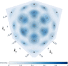Figure 2
Plot of $[\rho(\bf{k})]$ for a cubic lattice with a = 3 Å, $[l_{\max} = 6]$ , ten Bessel function radial basis functions. One can see that $[\rho(\bf{k})]$ attains its maximum values at reciprocal-lattice points.

To retain more information, we combine three sets of coefficients. The bispectrum b_l₁l₂l₃ is constructed by coupling coefficients from three channels (l₁,l₂,l₃) into a scalar quantity. To ensure invariance, the coupling is done through a symmetric Clebsch–Gordan tensor product (the same $[|l_{1}-l_{2}|\leq l_{3}\leq l_{1}+l_{2}]$ that governs angular momentum selection rules in quantum mechanics, see Section S5 and Section S7). The tensor product is also symmetrized over the indices (l₁,l₂,l₃), guaranteeing that the result is permutation invariant. Note that, to distinguish between structures related by inversion, one should include pseudoscalars along with the scalars from the coupling [corresponding to the O(3) group rather than the SO(3) group]. This is not necessary for Bravais lattices as they are centrosymmetric but is included here for completeness. The tensor product can be written as

$[{\bf B} = ({\bf c}_{l_{3}}\otimes({\bf c}_{l_{1}}\otimes {\bf c}_{l_{2}}))^{(0_{e}\oplus 0_{o})},\eqno(4)]$

where $[(0_{e}\oplus 0_{o})]$ emphasizes we are retaining the scalars and pseudoscalars. For N_r radial basis functions and maximum l_max, the final descriptor dimension is

$[{\rm dim}({\bf B}) = \left(N_{r},\sum_{l_{1} = 0}^{l_{\max}}\sum_{l_{2} = 0}^{l _{\max}}\sum_{l_{3} = 0}^{l_{\max}}N_{\rm {allowed}}(l_{1},l_{2},l_{3})\right),\eqno(5)]$

where $[N_{\rm {allowed}}(l_{1},l_{2},l_{3})]$ counts the number of scalar/pseudoscalar contributions after the two tensor products. In this representation, each row corresponds to a radial basis function n, and each column corresponds to an allowed coupling. This makes the bispectrum naturally visualizable as a 2D heatmap, as in Fig. 3.

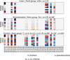Figure 3
Sample bispectra for crystal systems with varying levels of symmetry. Each column corresponds to a bispectrum component (l₁,l₂,l₃), grouped by angular channel. Scalar (e) and pseudoscalar (o) components are separated by the dashed line. All pseudoscalar components vanish, consistent with the centrosymmetry of Bravais lattices.

Because $[\rho({\bf k})]$ transforms equivariantly under the crystal's point group, only specific (l,m) channels can be non-zero. This is the same mathematical formalism that yields the first non-trivial charge-density multipole of a given lattice. For example, for a cubic lattice with O_h symmetry, only specific l channels ( $[l = 0,4,6,8,\ldots)]$ contribute to the lattice bispectrum. This is confirmed in Fig. 3. The sparsity pattern of the bispectrum directly reflects the underlying symmetry of the unit cell. Consequently, higher-symmetry lattices produce more zero entries. As unit cells retain the symmetry of a parallelepiped, the lattice bispectrum is constrained to have zeros in certain entries for all lattices (e.g. see the triclinic lattice in Fig. 3).

We enumerate the invariance properties of our construction of the reciprocal-lattice bispectrum. Following the construction of the bispectrum by Bartók et al. (2013), we obtain the bispectrum as symmetrized products of spherical harmonics coefficients (implemented using Clebsch–Gordan coefficients) in equation (4). It is therefore invariant under SO(3). If we include pseudoscalars, it then has components that change sign under inversion. (l₁,l₂,l₃) in equation (4) are invariant under inversion or accumulate a negative sign depending on whether l₁+l₂+l₃ is even or odd. However, every reciprocal lattice is centrosymmetric, so all odd combinations of l₁+l₂+l₃ are zero, and the descriptor is thus invariant under the O(3) group. We retain the pseudoscalar channels for generality. These invariances naturally align with the physics of powder diffraction. Rotation invariance means that the descriptor depends on relative geometry rather than absolute orientation. Inversion invariance is consistent with XRD as we measure the intensity in Fourier space $[|F({\bf G})|^{2}]$ at reciprocal-lattice points $[{\bf G}]$ , so we will have the same measurement if $[{\bf G}\to-{\bf G}]$ .

There are additional properties resulting from using the reciprocal-lattice vectors to construct the lattice bispectrum. The reciprocal lattice depends only on the real-space lattice vectors, which are unchanged by a translation of the crystal, so the descriptor does not depend on the choice of real-space origin. Moreover, any set of primitive lattice vectors will generate the same set of lattice points. As c_nlm is a sum over these points, the descriptor is independent of the choice of primitive cell, including permutations or re-indexing of the vectors $[\{{\bf b}_{1},{\bf b}_{2},{\bf b}_{3}\}]$ . These properties ensure that the descriptor encodes the geometric information of relative distances and angles between reciprocal-lattice points that determine the Bravais lattice. See Section S5.1 for the theoretical justification of the sparsity pattern in the bispectrum.

We note that this representation is motivated by the discontinuity that arises in lattice parameter representations under conventional space-group settings. Small continuous distortions of a lattice can trigger a change in the reduced-cell convention, producing artificial jumps even when the underlying geometry changes smoothly. This concept is illustrated in Fig. 4, which shows a cubic cell being uniformly distorted into a triclinic cell. Measured in the L² norm from the starting bispectrum, the bispectrum is seen to change smoothly throughout the distortion (modulo numerical artifacts). This representation has the advantage of producing smooth variations in the L² norm under continuous lattice deformations, instead of relying on reduced-cell-based representations such as S⁶, where distances between lattices are computed after a reduction step that can introduce non-uniqueness in the choice of basis (Andrews & Bernstein, 2023 ). As a result, such metrics can exhibit apparent non-smooth behavior along continuous deformation paths. See Fig. S3 for a sensitivity analysis of the inversion to Gaussian noise in the bispectrum.

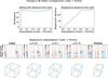Figure 4
Example interpolation between a cubic and triclinic lattice and the corresponding change in bispectrum and S⁶ distance. The interpolation parameter α linearly deforms the lattice in real space. While the bispectrum varies smoothly in the Euclidean ( L²) norm along this path, distances computed in reduced-cell representations (e.g. S⁶) can exhibit non-smooth behavior due to changes in the chosen reduced basis during lattice reduction. Note that intermediate lattices are also triclinic, as the interpolation does not enforce any symmetry constraints.

4.1.1. Practical details

In practice, this descriptor includes some hyperparameters that are user-defined. These include k_max, l_max, the type of radial basis function and the number of radial basis functions. k_max depends on the limiting resolution of the detector. For our purposes, we use the standard Cu Kα wavelength of 1.5406 Å. Note here we use the crystallographic convention common in XRD, so there is no factor of $[2\pi]$ . Assume that $[2\theta_{\max} = 60^{\circ}]$ , we then have $[k_{\max}\approx{{2} \over {3}}]$ Å⁻¹.

As we are modeling a periodic structure, in practice, we also want k_max large enough such that every reciprocal-lattice point within a certain radius of the Γ point is included in the descriptor at least once. For a unit cell, this is $[k_{\max}\ {\gtrsim}\ {(1 / a_{\min})}]$ where a_min is the smallest lattice parameter or equivalently $[k_{\max}\ {\gtrsim}\ { b_{\max}}]$ where b_max is the maximum reciprocal-lattice vector. As seen in Fig. 5, our cutoff does satisfy this condition for nearly all lattices in the Materials Project dataset. For different datasets, this could require further tuning.

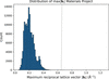Figure 5
Distribution of the magnitude of the maximum reciprocal-lattice vector (using the crystallographic convention) for the Materials Project dataset.

We find $[l_{\max} = 6]$ is sufficient to resolve angular lattice information, following standard atomic descriptor literature (Bartók et al., 2013). We choose to use Bessel functions as the radial basis function in order to assign higher weight to points near the Γ point, but to also allow for variation outside of a narrow envelope (as opposed to Gaussian basis functions) and use ten radial basis functions.

4.2. Inversion of the lattice bispectrum

We demonstrate how to invert the lattice bispectrum to obtain the lattice parameters (the second step in Fig. 1). While the bispectrum is not mathematically complete [i.e. it is not a one-to-one mapping; see Bendory et al. (2025 ) for generic uniqueness results], it can be empirically inverted (Nigam et al., 2026) in an auto-differentiable framework. We use a precomputed database of bispectra as a nearest-neighbor lookup to initialize the starting guess for the inversion. We show the approach in Fig. 6. We aim to invert the mapping $[f(a,b,c,\alpha,\beta,\gamma) = {\bf B}]$ to obtain lattice parameters $[(a,b,c,\alpha,\beta,\gamma)]$ , where f represents the bispectrum calculation. Crucially, f can be implemented in an auto-differentiable framework such as PyTorch (Paszke et al., 2019 ). Thus, standard optimization tools can be used to invert f. In practice, we found that second-order optimization methods such as L-BFGS-B [limited-memory Broyden–Fletcher–Goldfarb–Shanno (Byrd et al., 1995 )] provide more accurate lattice parameter predictions. Additionally, the starting lattice guess can improve convergence. Thus, we initialize $[v_{\rm {guess}} = (a,b,c,\alpha,\beta,\gamma)_{\rm {guess}}]$ using precalculated bispectra from the Materials Project database (with distance between bispectra measured by the L² norm). (One could also use other crystallographic databases. The calculated bispectra are available from https://github.com/atomicarchitects/bispectrum-xrd-ml/tree/main.) In practice, nearest entries by mean squared error are used as starting points. Each starting lattice is perturbed with Gaussian noise of standard deviation $[0.05\,\|{\bf L}^{*}\|_{F}]$ per element of the reciprocal-lattice matrix $[{\bf L}^{*}]$ and whose rows are $[{\bf b}_{1},{\bf b}_{2},{\bf b}_{3}]$ , and optimized with L-BFGS-B using SciPy (Virtanen et al., 2020 ). If a candidate reaches a bispectrum loss below $[10^{-3}]$ , no further candidates are tried; otherwise the lattice with the lowest loss is returned. Candidate selection uses only the predicted bispectrum. As the calculation of $[{\bf B}]$ is differentiable, one can then calculate a loss between $[{\bf B}]$ and the calculated bispectra, and then update $[v_{\rm {guess}}]$ based on this loss with an optimization step.

Figure 6
Algorithm to invert the lattice bispectrum. Given an initial bispectrum, the starting lattice parameters are initialized from the nearest entry in a precomputed database of bispectra. The residual between the true and predicted bispectra is then calculated and lattice parameters are updated with a L-BFGS step. After inversion, we obtain a set of vectors spanning the primitive lattice. Standard crystallographic tools such as pymatgen or cctbx can then be used for postprocessing.

4.3. Bispectrum prediction from XRD patterns

We use a transformer model to predict the lattice bispectrum from XRD patterns. We developed a hierarchical tokenization approach that segments the XRD pattern into overlapping local windows with a transformer-based architecture. This strategy succeeds at capturing relevant structural information across different scales while maintaining positional accuracy. After window extraction, each window is passed through a feedforward neural network. The resulting tokens are then refined with a multi-head self-attention mechanism. This methodology preserves positional precision that CNN-based approaches lose through pooling, yet also captures long-range angular dependencies. Model hyperparameters and training details are in Table S1 and the architecture is shown in Fig. 7.

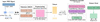Figure 7
Transformer model architecture used for predicting the bispectrum from XRD input.

5. Results

To test the utility of the lattice bispectrum as compared with directly predicting the lattice parameters, we first focus on the MP-20 dataset. In general, there is no widely established benchmarking dataset for the unit-cell prediction problem, as different works tend to use augmented versions of the Materials Project, ICSD or CSD databases. However, recent crystal structure generation studies (Xie et al., 2021; Riesel et al., 2024; Li et al., 2025) have used the MP-20 dataset. MP-20 consists of structures from the Materials Project with up to 20 atoms per unit cell, containing 45231 inorganic materials. This dataset has the advantage of having predefined train, validation and testing splits from Xie et al. (2021), making it suitable for benchmarking. We further explore the impact of data augmentation by incorporating physics-based XRD augmentations into the MP-20 dataset as described in Section 5.1.1. We then consider larger systems by using the full Materials Project dataset with the same physics-based augmentations (Section 5.2). In each section, we assess the advantages of the bispectrum lattice representation versus directly predicting lattice parameters by using the same model architecture [with either an output dimension of 6 for lattice parameters or $[{\rm dim}({\bf B})]$ for the bispectrum]. Results per dataset are shown in Table 1.

Table 1
MAE and MAPE per dataset for bispectrum + inversion and direct prediction of lattice parameters

MP-20 and MP-20 augmented (aug.) are evaluated on the MP-20 test set. MP-full and MP-full aug. are evaluated on the MP-full test set (so this represents a more difficult learning problem with a larger set of diverse structures). Note that the evaluations in this table are done using synthetic patterns. The best method for each dataset is in bold.

Training data (No. of patterns)	Method	Length MAE (Å)	Length MAPE (%)	Angle MAE (°)	Angle MAPE (%)	Volume MAPE (%)
MP-20 (27k)	Direct	0.69	11.08	10.77	12.15	24.86
MP-20 (27k)	Bispectrum + inversion	0.18	2.43	2.19	2.45	5.15
MP-20 aug. (270k)	Direct	0.80	13.20	12.36	13.33	27.96
MP-20 aug. (270k)	Bispectrum + inv.	0.23	3.19	2.58	2.90	6.61
MP-full (93k)	Direct	1.24	15.33	10.20	11.21	33.95
MP-full (93k)	Bispectrum + inv.	0.44	4.46	3.92	4.41	10.09
MP-full aug. (930k)	Direct	1.27	15.75	9.87	10.91	33.67
MP-full aug. (930k)	Bispectrum + inversion	0.62	6.35	5.27	5.94	14.25

Note that the bispectrum inversion procedure yields a set of vectors that span the lattice. Thus, we perform postprocessing steps using pymatgen and cctbx after the inversion in order to fairly compare our results with the true lattice. Both the true and predicted lattice are passed to cctbx, which finds the best-matching canonical representation. Lattice parameter errors are computed between the canonicalized true lattice for the direct prediction and bispectrum inversion. This ensures that errors are computed in a consistent setting.

We analyze direct versus bispectrum model performance on structures with dominant zones in the Materials Project database in Section 5.3. The performance of each method is compared with benchmark predictions from Crystalyze and from a newer AlphaDiffract model (Andrejevic et al., 2026) on RRUFF experimental data in Section 5.4.

5.1. MP-20

In alignment with previous work (Chitturi et al., 2021; Riesel et al., 2024), we report the mean absolute percentage error (MAPE) for angles, lengths and unit-cell volumes, defined as

$[{\rm MAPE} = {{|{\rm true}-{\rm predicted}|} \over {{\rm true}}}\times 100\eqno(6)]$

as well as the mean absolute error (MAE) per Bravais lattice. We first consider the MP-20 dataset used by Xie et al. (2021), with the same train/test/validation splits used. The bispectrum prediction outperforms directly predicting the lattice parameters across Bravais lattices (see Fig. 8), most likely due to the fact that the bispectrum more strictly obeys symmetry constraints. For example, without training a model for separate crystal systems as done by Chitturi et al. (2021), Shu et al. (2025), the direct predictions may yield slightly different angle or length values that do not align with the correct Bravais lattice. This effect is not observed in the bispectrum prediction, where angle predictions are symmetry constrained and snap to the correct unit cell. See Section S8.1 for additional results.

Figure 8
MAE for bispectrum + inversion compared with direct predictions per Bravais lattice for MP-20.

5.1.1. Augmented MP-20

In order to generalize to experimental XRD patterns, we augmented synthetic XRD patterns from MP-20 to mimic experimental data. We follow the work of Salgado et al. (2023 ), Szymanski et al. (2021 ), Riesel et al. (2024), which provide insight into physically informed data augmentation of synthetic XRD patterns. The resulting augmented spectra sample possible changes in peak positions, intensities and widths. (i) Shifts in peak positions ( $[2\theta]$ ) were created using strain tensors for small distortions that preserve the space group of the parent structure. Modified unit cells were created with up to ± 4% strain. (ii) Peak intensities were varied through randomly selecting Miller indices (hkl) and then scaling peak intensities by 50% of original values. (iii) Peak widths were augmented through varying the Caglioti parameters U,V,W (see Section S4), which parameterize the angular dependence of the full width at half-maximum (FWHM) of diffraction peaks via FWHM² = $[U\tan^{2}\theta+V\tan\theta+W]$ (Caglioti et al., 1958 ). Each structure was augmented three times per method, providing a diverse set of plausible XRD patterns. Following Riesel et al. (2024), background noise sampled from a Gamma distribution is also added dynamically during training. The training set then has 271360 examples instead of 27136 as with MP-20. Note that data augmentation is applied to the training set, but the model is evaluated on the same testing set as MP-20 to ensure a fair comparison. Full details are in Section S4. We again observe that the bispectrum outperforms the direct prediction method, with the relative improvement being slightly smaller (Figs. 9 –11).

Figure 9
MAE for bispectrum + inversion compared with direct predictions per Bravais lattice for MP-20 augmented.

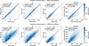Figure 10
Predicted versus true for a,b,c and volume for bispectrum + inversion and direct prediction of parameters using the MP-20 augmented dataset.

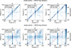Figure 11
Predicted versus true for $[\alpha,\beta,\gamma]$ for bispectrum + inversion and direct prediction of parameters using the MP-20 augmented dataset.

5.2. Augmented full Materials Project

Previous ML-XRD studies (Guo et al., 2025; Riesel et al., 2024) have rarely used the full Materials Project dataset. While the full Materials Project is invariably more complex than MP-20, we hypothesize that the greater diversity in crystal systems, unit-cell sizes and compositional complexity will lead to better generalization to structures with dominant zones. We create by reduced chemical formula a 60% training, 20% validation and 20% test split. A data leakage audit based on XRD-pattern similarity is given in Section S2.3. We apply the same physics-based augmentations as in Section 5.1.1 to the training set, resulting in a 930k pattern augmented dataset. This is a significantly more diverse dataset than MP-20 and thus represents a more difficult prediction problem. Nonetheless, we observe the same trend, with the bispectrum generally outperforming the direct predictions (Figs. 12 –14). Angle predictions are more difficult than length predictions with more diversity in unit cells, although this trend is not uniform across Bravais lattices (see Fig. S21). See Section S8.4 for additional per-Bravais lattice MAE and parity plots comparing bispectrum and direct prediction. Section S8.3 additionally contains results of training on the full Materials Project dataset without augmentation.

Figure 12
MAE for bispectrum + inversion compared with direct predictions per Bravais lattice using the MP full augmented dataset.

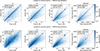Figure 13
Predicted versus true for a,b,c and volume for bispectrum + inversion and direct prediction of parameters using the MP full augmented dataset.

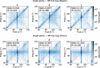Figure 14
Predicted versus true for $[\alpha,\beta,\gamma]$ for bispectrum + inversion and direct prediction of parameters using the MP full augmented dataset.

5.3. Dominant zones

A standard challenge in indexing pertains to dominant zone structures, in which most or all reflections can be indexed with two Miller indices (e.g. by h0l) (Schlesinger et al., 2022 ), usually where one axis in the unit cell is much larger than the others. We investigate the performance of the model trained on the full Materials Project data on dominant zone structures, comparing the bispectrum predictions with direct predictions of the lattice parameters. We define dominant zone patterns as powder diffraction patterns in which a large fraction of total intensity (≥ 50%) is indexed by reflections belonging to a single zero-index family (i.e. , or ). This provides a simple measure of indexing anisotropy in reciprocal space, capturing cases where diffraction intensity is strongly concentrated within coordinate-aligned Miller-index subspaces such as 00l, h0l or hk0. Note that we use a diffraction-based definition rather than considering real-space lattice anisotropy as lattice recovery from XRD patterns depends on reciprocal-space indexing. Using this criteria, 1100 out of 30000 structures in the test set were identified as dominant zone structures.

We find that the bispectrum prediction method performs much better on dominant zone structures (see Fig. 15). For instance, 76.6% of dominant zone structures have both length and angle MAPE less than 5% when predicting the lattice bispectrum. However, this is only the case for 5.8% of the direct parameter predictions. We hypothesize this advantage stems from the symmetry-preserving properties of the lattice bispectrum. Dominant zone structures concentrate diffraction information into a reduced subspace of Miller indices, leaving the remaining lattice geometry underconstrained by the pattern. Direct prediction must resolve this ambiguity within an unconstrained six-parameter space, whereas bispectrum inversion benefits from a representation that already encodes the lattice's symmetry constraints (Table 2).

Table 2
Dominant zone success metrics for direct prediction and bispectrum + inversion

Analysis was done using the MP-full test set and the MP-full aug. trained model. The best method is in bold.

Method	Fraction ≤ 5% length MAPE	Fraction ≤ 5% angle MAPE	Fraction both ≤ 5%
Direct	9.6%	47.5%	5.8%
Bispectrum + inversion	82.0%	81.7%	76.6%

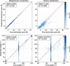Figure 15
Parity plots for dominant zone structures (MP full test set, MP full augmented model), for bispectrum inversion (left) and direct lattice parameter prediction (right). Top: predicted versus true dominant (longest) axis. Bottom: predicted versus true lattice angles (α, β, γ pooled); the columns at 90° and 120° are angles fixed by symmetry – bispectrum inversion largely preserves them, while direct prediction scatters them over 60–120°.

5.4. Experimental data and comparisons with benchmarks

Direct comparison across methods in this field is challenging due to inconsistent evaluation protocols, training datasets and test splits; where possible, we have attempted to ensure fair comparison by rerunning baseline models with identical postprocessing. In line with prior works (e.g. Riesel et al., 2024; Choudhary, 2025; Andrejevic et al., 2026), we consider the RRUFF dataset to test the generalization of our model to experimental data. First, we consider the same 134 RRUFF structures as used in Crystalyze (Riesel et al., 2024) in order to have a consistent benchmark. We obtain the predicted lattice parameters from the MP-20 augmented model evaluated on the Crystalyze RRUFF dataset. Crystalyze is a structure generation model that predicts composition, lattice parameters and number of atoms from an XRD pattern before denoising random atom positions to obtain a sampled structure. It is therefore a substantially more complex model than ours. We average output Crystalyze predictions over five sampled structures. As seen in Table 3, despite predicting only lattice parameters rather than full crystal structures, the bispectrum model achieves comparable performance with Crystalyze on experimental data. Additionally, our data augmentation strategy clearly aids in performance, as seen in Fig. 16 and Section S8.5.

Table 3
MAE and MAPE on RRUFF experimental data

We evaluate on the same 134-structure test set as Crystalyze, with all predictions postprocessed using cctbx to project onto the nearest valid Bravais lattice. Note these structures are filtered to be less than 20 atoms per unit cell. The best method for each dataset is in bold.

Training data	Method	Length MAE (Å)	Length MAPE (%)	Angle MAE (°)	Angle MAPE (%)	Volume MAPE (%)
MP-20 aug.	Crystalyze	0.90	16.08	8.74	9.93	43.37
MP-20 aug. (270k)	Direct (ours)	1.86	30.92	9.46	10.29	94.82
MP-20 aug. (270k)	Bispectrum + inversion (ours)	0.91	14.41	8.37	8.94	35.72

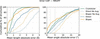Figure 16
Cumulative distribution function for length and angle MAE for the RRUFF Crystalyze test set. The dashed lines correspond to the model trained on the MP-20 dataset with no augmentation, and the solid lines correspond to the model trained on the MP-20 dataset with augmentation as described in Section 5.1.1

. Augmentation clearly improves performance.

We further compare the performance of our model with that of AlphaDiffract on the AlphaDiffract RRUFF test set. This is a different set of 240 RRUFF structures to those used by Crystalyze, as AlphaDiffract does not limit training data to less than 20 atoms per unit cell (Andrejevic et al., 2026). As seen in Table 4, our model underperforms AlphaDiffract, which is expected given that AlphaDiffract trains on 31 million patterns – 33× our training set size. Notably, training on 3% of AlphaDiffract's data, our bispectrum model approached comparable length MAE (2.50 versus 2.11 Å) though the angle error gap remains larger.

Table 4
MAE and MAPE on RRUFF AlphaDiffract experimental data

We evaluate on the same 240-structure test set as AlphaDiffract, with all predictions postprocessed using cctbx to project onto the nearest valid Bravais lattice.

Training data	Method	Length MAE (Å)	Length MAPE (%)	Angle MAE (°)	Angle MAPE (%)
AlphaDiffract MP-full (31M)	AlphaDiffract	2.11	23.50	2.72	2.91
MP-full aug. (930k)	Direct (ours)	4.36	50.75	8.76	9.39
MP-full aug. (930k)	Bispectrum + inversion (ours)	2.50	31.78	9.90	10.86

We also explored scaling the model by 1.5× and 2×, finding small improvements on the RRUFF AlphaDiffract set ( $[\approx 1^{\circ}]$ and $[\approx 2^{\circ}]$ , respectively, in angle improvement). This suggests that model capacity is not the primary bottleneck, and that closing the simulation-to-real gap requires larger or more diverse training data. On the RRUFF dataset, we observe that our data augmentation aids in performance (see Fig. 16), albeit not matching that of AlphaDiffract.

We additionally evaluate both the bispectrum and direct prediction models on a curated subset of single-phase patterns from the CNRS/COD (CNRS, Centre National de la Recherche Scientifique) contribution to the opXRD database (Hollarek et al., 2026 ). Both models show larger errors on this dataset than on RRUFF (Table 5). Following standard practice (Riesel et al., 2024), our noise augmentation was fitted to RRUFF. We hypothesize this differing performance is due to the background noise augmentation specifically being fitted to the RRUFF dataset. Exploratory ablations support this: retraining with CNRS-informed background noise alone substantially reduces error, and peak-list inputs lower the average length error further. Direct prediction also rarely recovers the full cell: on every experimental set, fewer than 5% of its predictions have both length and angle MAPE below 5%, whereas the bispectrum model trained with CNRS-informed noise reaches 25% on these patterns. This is an important caution for practitioners: models trained with noise augmentation fitted to one experimental dataset may not generalize to others. Identifying training procedures that generalize across experimental datasets is an important direction for future work (full results in Section S8.6).

Table 5
MAE and MAPE on CNRS opXRD patterns with at most 20 atoms per primitive cell, for models trained on MP-20 aug. and postprocessed with cctbx

All rows use the same patterns. `+ CNRS noise': background noise informed by CNRS patterns during training; `Peak list': up to 30 extracted peaks as input. Best value per column in bold. Full results, including MP-full aug. and RRUFF, are in Table S5.

Training data	Method	Length MAE (Å)	Length MAPE (%)	Angle MAE (°)	Angle MAPE (%)
MP-20 aug. Dense	Direct	2.15	39.17	8.26	8.88
MP-20 aug. Dense	Bispectrum + inversion	2.54	43.36	13.85	14.95
MP-20 aug. Dense + CNRS noise	Bispectrum + inversion	1.62	26.60	10.87	11.67
MP-20 aug. Peak list + CNRS noise	Direct	1.59	26.37	10.66	11.40
MP-20 aug. Peak list + CNRS noise	Bispectrum + inversion	1.14	17.34	9.49	10.01

6. Related literature

The following references are cited in the supporting information: Altmann & Herzig (1994 ), Bendory et al. (2018 ), Cobelli et al. (2022 ), Dresselhaus et al. (2008 ), Geiger & Smidt (2022 ), Kakarala (2012 ), Nigam et al. (2023 ), Pinilla et al. (2023 ), Pozdnyakov et al. (2020 ).

7. Discussion

We develop an invertible unit-cell representation in reciprocal space. Crucially, this is invariant to the choice of primitive unit cell. While previous ML approaches to predicting lattice parameters from XRD patterns have not taken the unit-cell representation into account, we hypothesize that our geometry-informed representation will lead to more robust predictions. We test our hypothesis using a transformer-based architecture. We find that the bispectrum representation aids in predictions for both the MP-20 and the full Materials Project dataset for simulated XRD patterns.

The bispectrum acts to eliminate the ambiguity of reduced-cell conventions. When predicting lattice parameters correctly, the model must implicitly learn a single consistent convention, whereas the training data may contain equivalent cells expressed differently. Second, the bispectrum naturally enforces symmetry constraints. As shown in Fig. 3, higher-symmetry lattices produce sparser bispectra, and the inversion procedure recovers lattice parameters that respect these constraints without requiring separate per-crystal models as in prior work. In contrast, with direct prediction, angles or lengths are more likely to deviate slightly from their symmetry-constrained values (e.g. predicting cubic angles that are not exactly 90°). Third, the bispectrum varies smoothly under continuous lattice deformations, whereas reduced-cell parameters can change discontinuously at symmetry boundaries. This may produce a more learnable loss landscape for the neural network.

Several limitations should be noted. The inversion step adds computational overhead (a median of 88 s per structure on a single CPU core with 15 starting candidates; see Section S3.4) but is parallelizable. With more difficult experimental patterns that are out of distribution of the training data, bispectrum predictions are further from the ground truth. Thus, inversion becomes more difficult and can lead to degradation of the predicted lattice parameters (see Fig. S4). Performance on experimental data remains below that on synthetic data, reflecting the well documented simulation-to-real gap. Closing this gap will likely require a much larger dataset and augmentation strategies that better capture the full range of experimental artifacts, as done by Andrejevic et al. (2026), which is beyond the scope of this work. Additionally, our augmentation strategy, while physically motivated, is a simplification of real experimental variability (see Section S4.1).

A general obstacle to progress in this area is the absence of a standardized augmentation and evaluation protocol. Throughout this work, we have tried to make comparisons fair by matching test splits and postprocessing pipelines to prior methods where feasible. We believe the community would benefit from a shared benchmark dataset analogous to MP-20 and collecting experimental data, much of which is scattered across personal repositories. This would ideally fix the training corpus, augmentation protocol and evaluation split so that lattice parameter prediction methods can be compared directly.

In terms of future work, the lattice bispectrum could serve as a useful intermediate representation for other crystallographic ML tasks. For example, structure generation models such as Crystalyze could potentially benefit from conditioning on the bispectrum rather than on raw lattice parameters. Additionally, we note that our model is predictive as it outputs lattice parameters given an XRD pattern. An interesting avenue for future work would be to extend our approach to be generative to sample candidate lattice parameters. This could represent a more faithful formulation of the XRD to lattice parameter problem, as it is fundamentally a one-to-many mapping. An interesting extension of the lattice bispectrum could be to incorporate the structure factor, yielding an atomic descriptor sensitive to both the lattice geometry and the atomic basis. This could aid in full structure determination beyond solely lattice parameters.

Supporting information

Supporting information for the main text (computational details, additional numerical experiments, and theoretical background). DOI: https://doi.org/10.1107/S2053273326010284/zi5012sup1.pdf

Acknowledgements

We thank Nina Andrejevic for helpful information about AlphaDiffract and Eric Riesel for discussions regarding Crystalyze. We also thank Emily Oliphant and Ameya Daigavane for helpful discussions regarding our methodology. This report was prepared as an account of work sponsored by an agency of the United States Government. Neither the United States Government nor any agency thereof, nor any of their employees, makes any warranty, express or implied, or assumes any legal liability or responsibility for the accuracy, completeness, or usefulness of any information, apparatus, product, or process disclosed, or represents that its use would not infringe privately owned rights. Reference herein to any specific commercial product, process, or service by trade name, trademark, manufacturer, or otherwise does not necessarily constitute or imply its endorsement, recommendation, or favoring by the United States Government or any agency thereof. The views and opinions of authors expressed herein do not necessarily state or reflect those of the United States Government or any agency thereof.

Conflict of interest

There are no known conflicts of interests.

Data availability

We have made the code available at https://github.com/atomicarchitects/bispectrum-xrd-ml including the Materials Project identifiers for all dataset splits and the identifiers of the RRUFF/CNRS subsets.

Funding information

EH was supported by the US Department of Energy, Office of Science, Office of Advanced Scientific Computing Research, Department of Energy Computational Science Graduate Fellowship under award No. DE-SC0024386. The National Institutes of Health, National Institute of General Medical Sciences supported DWMM and DWP via grant R24GM154040 to ASB. This research used resources of the National Energy Research Scientific Computing Center (NERSC), a Department of Energy User Facility using NERSC awards ERCAP0033254 and ERCAP0036437. The authors also gratefully acknowledge the support by the Department of Energy Office of Science under the ICDI (Integrated Computational and Data Infrastructure) grant DE-SC0022215 and the Air Force Office of Scientific Research under award No. FA9550-24-1-0067.

References

Altmann, S. L. & Herzig, P. (1994). Point-Group Theory Tables. Oxford: Clarendon Press. Google Scholar
Andrejevic, N., Du, M., Sharma, H., Horwath, J. P., Luo, A., Yin, X., Prince, M., Toby, B. H. & Cherukara, M. J. (2026). AlphaDiffract: Automated Crystallographic Analysis of Powder X-ray Diffraction Data. arXiv:2603.23367. Google Scholar
Andrews, L. C. & Bernstein, H. J. (2014). J. Appl. Cryst. 47, 346–359. Web of Science CrossRef CAS IUCr Journals Google Scholar
Andrews, L. C. & Bernstein, H. J. (2023). arXiv:2302.10240. Google Scholar
Andrews, L. C., Bernstein, H. J. & Sauter, N. K. (2019). Acta Cryst. A75, 593–599. CrossRef IUCr Journals Google Scholar
Bartók, A. P., Kondor, R. & Csányi, G. (2013). Phys. Rev. B 87, 184115. Google Scholar
Bendory, T., Boumal, N., Ma, C., Zhao, Z. & Singer, A. (2018). IEEE Trans. Signal Process. 66, 1037–1050. CrossRef Google Scholar
Bendory, T., Edidin, D., Katz, J. & Kreymer, S. (2025). arXiv:2508.02674. Google Scholar
Boultif, A. & Louër, D. (1991). J. Appl. Cryst. 24, 987–993. CrossRef CAS IUCr Journals Google Scholar
Byrd, R. H., Lu, P., Nocedal, J. & Zhu, C. (1995). SIAM J. Sci. Comput. 16, 1190–1208. CrossRef Google Scholar
Caglioti, G., Paoletti, A. & Ricci, F. P. (1958). Nucl. Instrum. 3, 223–228. CrossRef CAS Web of Science Google Scholar
Chitturi, S. R., Ratner, D., Walroth, R. C., Thampy, V., Reed, E. J., Dunne, M., Tassone, C. J. & Stone, K. H. (2021). J. Appl. Cryst. 54, 1799–1810. CrossRef CAS IUCr Journals Google Scholar
Choudhary, K. (2025). J. Phys. Chem. Lett. 16, 2110–2119. CrossRef CAS Google Scholar
Cobelli, M., Cahalane, P. & Sanvito, S. (2022). Phys. Rev. B 106, 035402. Google Scholar
Coelho, A. A. (2003). J. Appl. Cryst. 36, 86–95. Web of Science CrossRef CAS IUCr Journals Google Scholar
Coelho, A. A. (2017). J. Appl. Cryst. 50, 1323–1330. Web of Science CrossRef CAS IUCr Journals Google Scholar
Corriero, N., Rizzi, R., Settembre, G., Del Buono, N. & Diacono, D. (2023). J. Appl. Cryst. 56, 409–419. CrossRef CAS IUCr Journals Google Scholar
David, W. I. F. & Shankland, K. (2008). Acta Cryst. A64, 52–64. Web of Science CrossRef CAS IUCr Journals Google Scholar
De Wolff, P. M. (1957). Acta Cryst. 10, 590–595. CrossRef IUCr Journals Google Scholar
Dong, H., Butler, K. T., Matras, D., Price, S. W., Odarchenko, Y., Khatry, R., Thompson, A., Middelkoop, V., Jacques, S. D., Beale, A. M. & Vamvakeros, A. (2021). npj Comput. Mater. 7, 74. Web of Science CrossRef Google Scholar
Dresselhaus, M. S., Dresselhaus, G. & Jorio, A. (2008). Group Theory: Application to the Physics of Condensed Matter. Berlin: Springer. Google Scholar
Geiger, M. & Smidt, T. (2022). arXiv:2207.09453. Google Scholar
Gómez-Peralta, J. I., Bokhimi, X. & Quintana, P. (2023). J. Phys. Chem. A 127, 7655–7664. Google Scholar
Gómez-Peralta, J. I., Bokhimi, X. & Quintana-Owen, P. (2025). Scr. Mater. 263, 116697. Google Scholar
Grosse-Kunstleve, R. W., Sauter, N. K., Moriarty, N. W. & Adams, P. D. (2002). J. Appl. Cryst. 35, 126–136. Web of Science CrossRef CAS IUCr Journals Google Scholar
Guo, G., Saidi, T. L., Terban, M. W., Valsecchi, M., Billinge, S. J. L. & Lipson, H. (2025). Nat. Mater. 24, 1726–1734. Web of Science CrossRef CAS PubMed Google Scholar
Habershon, S., Cheung, E. Y., Harris, K. D. & Johnston, R. L. (2004). J. Phys. Chem. A 108, 711–716. CrossRef CAS Google Scholar
Harris, K. D. M. (2022). Acta Cryst. B78, 96–99. Web of Science CrossRef IUCr Journals Google Scholar
Hollarek, D., Schopmans, H., Östreicher, J., Teufel, J., Cao, B., Alwen, A., Schweidler, S., Singh, M., Kodalle, T., Hu, H., Heymans, G., Abdelsamie, M., Hardiagon, A., Wieczorek, A., Zhuk, S., Schwaiger, R., Siol, S., Coudert, F.-X., Wolf, M., Sutter–Fella, C. M., Breitung, B., Hodge, A. M., Zhang, T. & Friederich, P. (2026). Adv. Intell. Discov. 2, e202500044. . CrossRef Google Scholar
Horton, M. K., Huck, P., Yang, R. X., Munro, J. M., Dwaraknath, S., Ganose, A. M., Kingsbury, R. S., Wen, M., Shen, J. X., Mathis, T. S., Kaplan, A. D., Berket, K., Riebesell, J., George, J., Rosen, A. S., Spotte-Smith, E. W. C., McDermott, M. J., Cohen, O. A., Dunn, A., Kuner, M. C., Rignanese, G.-M., Petretto, G., Waroquiers, D., Griffin, S. M., Neaton, J. B., Chrzan, D. C., Asta, M., Hautier, G., Cholia, S., Ceder, G., Ong, S. P., Jain, A. & Persson, K. A. (2025). Nat. Mater. 24, 1522–1532. CrossRef CAS Google Scholar
Jain, A., Ong, S. P., Hautier, G., Chen, W., Richards, W. D., Dacek, S., Cholia, S., Gunter, D., Skinner, D., Ceder, G. & Persson, K. A. (2013). APL Mater. 1, 011002. Google Scholar
Kakarala, R. (2012). J. Math. Imaging Vis. 44, 341–353. CrossRef Google Scholar
Lafuente, B., Downs, R. T., Yang, H. & Stone, N. (2015). Highlights in Mineralogical Crystallography, edited by T. Armbruster & R. M. Danisi, pp. 1–30. Berlin: De Gruyter. Google Scholar
Lee, B. D., Lee, J.-W., Ahn, J., Kim, S., Park, W. B. & Sohn, K.-S. (2023). Adv. Intell. Syst. 5, 2300140. Web of Science CrossRef Google Scholar
Li, Q., Jiao, R., Wu, L., Zhu, T., Huang, W., Jin, S., Liu, Y., Weng, H. & Chen, X. (2025). Nat. Commun. 16, 7428. CrossRef Google Scholar
Li, Y., Yang, W., Dong, R. & Hu, J. (2021). ACS Omega 6, 11585–11594. CrossRef CAS Google Scholar
Mighell, A. D. (2000). Powder Diffr. 15, 82–85. Web of Science CrossRef CAS Google Scholar
Nigam, J., Phung, T., Daigavane, A., Tehrani, A. M. & Smidt, T. (2026). arXiv:2607.20338. Google Scholar
Nigam, J., Pozdnyakov, S. N., Huguenin-Dumittan, K. K. & Ceriotti, M. (2023). arXiv:2302.14770v1. Google Scholar
Ong, S. P., Richards, W. D., Jain, A., Hautier, G., Kocher, M., Cholia, S., Gunter, D., Chevrier, V. L., Persson, K. A. & Ceder, G. (2013). Comput. Mater. Sci. 68, 314–319. Web of Science CrossRef CAS Google Scholar
Paszke, A., Gross, S., Massa, F., Lerer, A., Bradbury, J., Chanan, G., Killeen, T., Lin, Z., Gimelshein, N., Antiga, L., Desmaison, A., Köpf, A., Yang, E., DeVito, Z., Raison, M., Tejani, A., Chilamkurthy, S., Steiner, B., Fang, L., Bai, J. & Chintala, S. (2019). Advances in Neural Information Processing Systems 32 (NeurIPS 2019). Google Scholar
Pinilla, S., Mishra, K. V. & Sadler, B. M. (2023). ICASSP 2023-2023 IEEE International Conference on Acoustics, Speech and Signal Processing (ICASSP), pp. 1–5. Google Scholar
Pozdnyakov, S. N., Willatt, M. J., Bartók, A. P., Ortner, C., Csányi, G. & Ceriotti, M. (2020). arXiv:2001.11696v2. Google Scholar
Riesel, E. A., Mackey, T., Nilforoshan, H., Xu, M., Badding, C. K., Altman, A. B., Leskovec, J. & Freedman, D. E. (2024). J. Am. Chem. Soc. 146, 30340–30348. CrossRef CAS Google Scholar
Salgado, J. E., Lerman, S., Du, Z., Xu, C. & Abdolrahim, N. (2023). npj Comput. Mater. 9, 214. Web of Science CrossRef Google Scholar
Schlesinger, C., Fitterer, A., Buchsbaum, C., Habermehl, S., Chierotti, M. R., Nervi, C. & Schmidt, M. U. (2022). IUCrJ 9, 406–424. CrossRef CAS IUCr Journals Google Scholar
Segal, N., Li, M., Miller, B. K. & Gómez-Bombarelli, R. (2026). arXiv:2606.14003. Google Scholar
Segal, N., Subramanian, A., Li, M., Miller, B. K. & Gomez-Bombarelli, R. (2025). arXiv:2512.04036. Google Scholar
Shu, K., Gui, D.-Y., Yan, W.-X. & Wang, C.-H. (2025). J. Chem. Inf. Model. 65, 10025–10036. CrossRef CAS Google Scholar
Suzuki, Y., Hino, H., Hawai, T., Saito, K., Kotsugi, M. & Ono, K. (2020). Sci Rep, 10, 21790. Google Scholar
Szymanski, N. J., Bartel, C. J., Zeng, Y., Tu, Q. & Ceder, G. (2021). Chem. Mater. 33, 4204–4215. . Web of Science CrossRef CAS Google Scholar
Virtanen, P., Gommers, R., Oliphant, T. E., Haberland, M., Reddy, T., Cournapeau, D., Burovski, E., Peterson, P., Weckesser, W., Bright, J., van der Walt, S. J., Brett, M., Wilson, J., Millman, K. J., Mayorov, N., Nelson, A. R. J., Jones, E., Kern, R., Larson, E., Carey, C. J., Polat, İ., Feng, Y., Moore, E. W., VanderPlas, J., Laxalde, D., Perktold, J., Cimrman, R., Henriksen, I., Quintero, E. A., Harris, C. R., Archibald, A. M., Ribeiro, A. H., Pedregosa, F., van Mulbregt, P., Vijaykumar, A., Bardelli, A. P., Rothberg, A., Hilboll, A., Kloeckner, A., Scopatz, A., Lee, A., Rokem, A., Woods, C. N., Fulton, C., Masson, C., Häggström, C., Fitzgerald, C., Nicholson, D. A., Hagen, D. R., Pasechnik, D. V., Olivetti, E., Martin, E., Wieser, E., Silva, F., Lenders, F., Wilhelm, F., Young, G., Price, G. A., Ingold, G., Allen, G. E., Lee, G. R., Audren, H., Probst, I., Dietrich, J. P., Silterra, J., Webber, J. T., Slavič, J., Nothman, J., Buchner, J., Kulick, J., Schönberger, J. L., de Miranda Cardoso, J. V., Reimer, J., Harrington, J., Rodríguez, J. L. C., Nunez-Iglesias, J., Kuczynski, J., Tritz, K., Thoma, M., Newville, M., Kümmerer, M., Bolingbroke, M., Tartre, M., Pak, M., Smith, N. J., Nowaczyk, N., Shebanov, N., Pavlyk, O., Brodtkorb, P. A., Lee, P., McGibbon, R. T., Feldbauer, R., Lewis, S., Tygier, S., Sievert, S., Vigna, S., Peterson, S., More, S., Pudlik, T., Oshima, T., Pingel, T. J., Robitaille, T. P., Spura, T., Jones, T. R., Cera, T., Leslie, T., Zito, T., Krauss, T., Upadhyay, U., Halchenko, Y. O. & Vázquez-Baeza, Y. (2020). Nat. Methods 17, 261–272. Web of Science CrossRef CAS PubMed Google Scholar
Visser, J. W. (1969). J. Appl. Cryst. 2, 89–95. CrossRef CAS IUCr Journals Web of Science Google Scholar
Xie, T., Fu, X., Ganea, O.-E., Barzilay, R. & Jaakkola, T. (2021). arXiv:2110.06197. Google Scholar

This is an open-access article distributed under the terms of the Creative Commons Attribution (CC-BY) Licence, which permits unrestricted use, distribution, and reproduction in any medium, provided the original authors and source are cited.

FOUNDATIONS
ADVANCES

ISSN: 2053-2733

Volume 83| Part 1| January 2027|

https://doi.org/10.1107/S2053273326010284

Open

access

Format		BIBTeX
		EndNote
		RefMan
		Refer
		Medline
		CIF
		SGML
		Plain Text
		Text

Format		BIBTeX
		EndNote
		RefMan
		Refer
		Medline
		CIF
		SGML
		Plain Text
		Text

research papers\(\def\hfill{\hskip 5em}\def\hfil{\hskip 3em}\def\eqno#1{\hfil {#1}}\)

Learning lattice parameters from powder X-ray diffraction data using invariants

1. Introduction

2. Background

2.1. Traditional indexing methods

3. Related work

3.1. Classifying lattice symmetries from XRD

3.2. Predicting lattice parameters

3.3. Structure generation

4. Methodology

4.1. Bispectrum lattice descriptor

4.1.1. Practical details

4.2. Inversion of the lattice bispectrum

4.3. Bispectrum prediction from XRD patterns

5. Results

5.1. MP-20

5.1.1. Augmented MP-20

5.2. Augmented full Materials Project

5.3. Dominant zones

5.4. Experimental data and comparisons with benchmarks

6. Related literature

7. Discussion

Supporting information

Acknowledgements

Conflict of interest

Data availability

Funding information

References

research papers