Dynamical refinement against 3D-ED data in Olex2–AutoChem using the N-Beam approach

Dynamical diffraction effects, long recognized as a complicating factor in the analysis of crystal structures based on electron diffraction data, can now be modelled directly within Olex2–AutoChem [Dolomanov et al. (2009). J. Appl. Cryst. 42, 339–341] when using diffraction data processed with the Rigaku CrysAlisPro data reduction software. The newly implemented N-Beam refinement approach, based on the Bloch-wave formalism, integrates seamlessly with the AutoChem [Matsumoto et al. (2021). J. Chem. Crystallogr. 51, 438–450] interface that links CrysAlisPro and Olex2. Fully integrated intensities derived from rotation electron diffraction experiments can be refined dynamically, yielding improved structure models and enabling the determination of absolute structure configuration from electron diffraction data. The workflow provides a direct, accessible route from experiment to dynamical refinement within a familiar software environment.

1. Introduction

3D electron diffraction (3D-ED) has matured into a powerful technique for determining single-crystal structures of sub-micrometre crystals across a wide range of chemical materials. The strong interaction between electrons and the crystal potential makes dynamical scattering significant. The relatively flat Ewald sphere at electron wavelengths helps in ensuring that many reciprocal-lattice points are simultaneously on (or near) diffraction positions, a requirement for dynamical intensity redistribution to occur. Together, these factors make kinematical refinement a poor approximation for electron diffraction data, resulting in high R factors and systematically biased structural parameters.

Dynamical refinement methods based on the Bloch-wave formalism (Bethe, 1928; Hirsch et al., 1977) address these limitations by explicitly modelling multiple scattering. Implementations in Jana2006/Dyngo (Palatinus et al., 2013; Palatinus et al., 2015; Palatinus et al., 2019), Felix (Cleverley & Beanland, 2022; Beanland et al., 2019) and ReciPro (Seto & Ohtsuka, 2022) have demonstrated the power of this approach, achieving accurate structure determination and enabling absolute configuration assignment from 3D-ED data. However, these implementations require specialized software and close coupling with specific data reduction pipelines [typically PETS (Palatinus et al., 2019)], which presents a barrier to widespread adoption. Integration into the Crys­AlisPro → Olex2 workflow, already familiar to X-ray crystallographers and increasingly used for electron diffraction, addresses this limitation. Here, we describe the implementation of the N-Beam dynamical refinement engine within Olex2–AutoChem (Dolomanov et al., 2009), which operates directly on fully integrated reflection intensities produced by CrysAlisPro. The method combines computational efficiency – using local beam neighbourhoods rather than full virtual-frame simulations – with seamless integration into the AutoChem interface (Matsumoto et al., 2021). This enables routine dynamical refinement, significantly reducing R factors, improving structural accuracy and reliably determining absolute stereochemistry for chiral molecules. The complete workflow from data collection to publication-quality structure determination can be completed in a few hours on standard desktop hardware, making dynamical refinement easily accessible.

2. Workflow integration

The N-Beam dynamical refinement engine is integrated into the established CrysAlisPro → Olex2 → AutoChem workflow, providing a seamless path from data collection to publication-quality structure determination. This section outlines the complete workflow and highlights the technical requirements that make dynamical refinement practical for routine use.

2.1. Data collection and integration

CrysAlisPro controls the data collection experiment on the Synergy-ED electron diffractometer (Ito et al., 2021) and performs reflection integration using algorithms adapted from XDS (Kabsch, 1988; Kabsch, 2010a; Kabsch, 2010b). Diffraction pixels are remapped into an undistorted coordinate space (`Kabsch space'), where reflections adopt similar profiles regardless of their measurement conditions – detector position, distance, angle or elevation relative to the rotation axis.

Integration is preceded by learning cycles that optimize profile shapes, crystal orientation and the instrument model to achieve the best agreement between predicted and observed reflection positions. Systematic effects such as beam incidence angles and electron-optical aberrations (ellipticity, barrel distortion, pincushion distortion) are corrected on a per-pixel basis. Additional corrections can account for sample wobbling, continuous movement, discrete jumps and position-dependent profile variations.

This level of geometric accuracy is essential for dynamical refinement: Bloch-wave intensity calculations critically depend on the precise knowledge of reflection positions and lattice orientation. Small errors in the orientation matrix or detector model propagate directly into errors in the calculated dynamical intensities.

All the information required to perform dynamical refinement is written to an extended CIF that contains not only the integrated intensities and standard crystallographic metadata but also the scan-space limits and integration boundaries for each reflection. This extended format preserves all information needed to reconstruct the measurement geometry for each reflection during N-Beam calculations.

The CIF is passed directly to Olex2 via the AutoChem interface, eliminating the need for manual file conversion or intermediate processing steps. This seamless data transfer is a key advantage of the integrated workflow: users work entirely within familiar software environments without needing to learn specialized dynamical refinement tools.

2.2. Structure solution and kinematical model refinement

Structure solution in Olex2 proceeds using standard methods for structure solution and atom-type assignment. The resulting model is then refined kinematically using electron scattering factors (Peng, 1999). The resulting model typically exhibits high R₁ values, limited by unmodelled dynamical effects.

This kinematical model – complete with anisotropic displacement parameters and geometrically placed hydrogen atoms at neutron distances (Allen & Bruno, 2010) – serves as the starting point for N-Beam dynamical refinement. It is important to ensure that the kinematical model is chemically sensible and as complete as possible before initiating dynamical refinement cycles.

2.3. Dynamical model refinement

Once the kinematical model is established, N-Beam refinement within olex2.refine (Bourhis et al., 2015) can be activated. The refinement engine computes dynamical intensities based on the current model () using the Bloch-wave formalism described in Section 3, and refines structural parameters (coordinates, displacement parameters, occupancies) against the observed intensities () using standard least-squares methods.

The transition from kinematical to dynamical refinement typically reduces R₁ from 15–30% to values below 15%, often reaching 5–10% for high-quality datasets (Palatinus et al., 2015; Palatinus et al., 2015; Cleverley & Beanland, 2023). Residual density maps¹ are significantly improved, and systematic errors in bond lengths and angles are reduced (Palatinus et al., 2017; Klar et al., 2023). For chiral structures, the absolute configuration can often be reliably determined (Brázda et al., 2019; Klar et al., 2023) (Section 4).

The entire workflow, from data collection to dynamical refinement, can be completed reasonably quickly (in the order of hours), making dynamical refinement practical for routine structural characterization rather than a specialized technique reserved for particularly challenging problems.

3. The N-Beam approach

The N-Beam approach is a computationally efficient implementation of the Bloch-wave formalism. The term N-Beam is used throughout this paper to refer specifically to our local-neighbourhood implementation: for each parent reflection, a structure matrix of dimension (N+1)×(N+1) is assembled from the N most strongly coupled neighbouring beams, selected by the criterion (Section 3.1). This differs from the classical N-beam formalism, in which a single structure matrix encompasses all reciprocal-lattice points simultaneously near the Ewald sphere; our approach is a computationally efficient approximation that trades completeness for speed, and has been validated to converge rapidly with increasing N (Appendix B). The basic formulae used in this work follow Palatinus et al. (2015).

To calculate dynamical intensities, the following steps are required:

(1) The periodic crystal potential measured in volts can be expressed as a crystal structure factor multiplied by a constant and scaled with the unit-cell volume (Zou et al., 2011),

where h is the Planck constant, m₀ the electron rest mass, e the electron charge and Ω the unit-cell volume. In crystallography, the reciprocal-lattice vector is usually denoted by ; in most electron microscopy and electron diffraction publications, the same vector is denoted by , and we will follow this notation. Moreover, constructive interference from a specific set of parallel atomic planes in a crystal lattice is a `reflection' in crystallography, but in electron microscopy it is called a `beam'. We use both terms synonymously.

The Bloch-wave formalism requires the use of a U_g potential, sometimes referred to as `scaled optical potentials' (Seto & Ohtsuka, 2022), in a form defined as (Hirsch et al., 1977; Zou et al., 2011)

where m is the relativistically corrected electron mass and are the Fourier coefficients of the electrostatic potential in volts [often denoted as V_g; here we aim to be consistent with equation (1)]. The final formula to calculate the crystal scaled optical potentials U_g based on the electron structure factor F_g (Å) is given as

where is a reciprocal-lattice vector, F_g are the Fourier components of the crystal in Å [and can be calculated on the basis of the structure model and electron atomic scattering factors (Peng, 1999)] and γ is the relativistic factor ( m/m₀) dependent on the electron energy [1.3914 for a 200 kV microscope, Table A.4.1 of Hirsch et al. (1977)]. These potentials quantify the strength of scattering into each diffracted beam.

(2) The (N+1)×(N+1) structure matrix is assembled for each observed beam. Off-diagonal elements are the crystal potentials U_gi coupling the beam (parent beam) to its neighbours , weighted by the obliquity correction factors m_gi. The diagonal elements of the matrix encode the excitation errors S_g,

scaled by . The excitation error S_g is a deviation from the exact Bragg condition and can be defined as the distance between a reciprocal-lattice point and the Ewald sphere. The factors m_gi account for the geometry of the crystal surface via the surface normal and the reciprocal-lattice vectors at the current rotation step:

The iterator i identifies any given hkl reflection used in this computation step. The electron wavevector inside the crystal (primary beam) is denoted as , while K_n is a scalar, the result of a dot product between the surface normal vector, directing towards the source of electrons, and the incident beam vector ().

(3) For a given sample thickness t, the scattering matrix is computed via eigenvalue decomposition , yielding .

(4) The dynamical intensity profile of the parent beam is evaluated by computing the intensity over a certain range around the ideal excitation spot () of the parent beam. Within this span, the intensity rocking-curve point is extracted from the first column and the first non-diagonal element of at each angular step. The integrated dynamical intensity is obtained by integrating partial intensities along S_g1.

(5) Steps (2) through (4) are repeated across a defined angular range around the ideal excitation condition () of the parent beam, updating the vector-dependent elements of – and hence performing a new eigenvalue decomposition – at each step, to build up the full dynamical rocking-curve profile from which the integrated intensity is extracted.

Our implementation focuses on selecting beams for a given structure matrix and extracting the dynamical intensity only for the beam for which neighbourhood reflections and the calculation step have been established. With the N-Beam approach, each reflection (the parent beam) is considered together with a selected set of neighbouring beams that contribute significantly to energy redistribution. The final dynamical intensity of each parent beam can thereby be estimated from a dynamical intensity plot and then used in the standard least-squares refinement of the structural parameters. A summary of our implementation of the N-Beam approach is presented in Fig. 1.

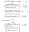Figure 1 Scheme 1. The flowchart of the N-Beam approach. Summary of relevant computation steps.

Note that kinematically forbidden reflections can carry significant dynamically scattered intensity. Olex2 therefore provides an option to include systematically absent reflections in the beam neighbourhood, with their contributions evaluated directly using the dynamical structure matrix.

3.1. Beam selection

The central step in our N-Beam approach is selecting which reflections to take into consideration for each parent beam. This selection must balance computational efficiency with physical accuracy: too few neighbours underestimate dynamical redistribution, while too many increase calculation time without improving results.

3.1.1. Physical context

In principle, only reflections simultaneously excited – those on or very near the Ewald sphere at the same moment – participate in multiple scattering. The excitation error S_g, evaluated at the near-Bragg angle of reflection g, measures the distance between a reciprocal-lattice point and the Ewald sphere along the vector . Reflections with are strongly excited and couple most efficiently, but reflections with small non-zero also contribute: for a crystal of finite thickness t, significant scattering intensity extends over a range of S_g related to 1/t around the exact Bragg condition.

The challenge is to identify, for each parent beam, the N neighbouring reflections that contribute most significantly to intensity redistribution. Two competing factors determine coupling strength:

Proximity to excitation: beams with smaller couple more strongly (geometric factor).

Scattering strength: beams with larger structure-factor amplitudes transfer more intensity (physical factor).

3.1.2. Selection criterion

We use the ratio as the primary selection criterion [similarly to Zuo & Weickenmeier (1995)], which naturally balances these competing effects. This prioritizes strong reflections, even if somewhat farther from exact excitation, and includes weak reflections only if very close to excitation.

To construct the neighbourhood for a given parent beam, a candidate list is assembled which includes all reflections (observed and unobserved) that satisfy the threshold criteria for the resolution limit, the maximum excitation error and the angular separation from the parent beam in rotation space. This list is then sorted by , and the top N reflections are selected as coupling partners. The optimum value of N depends on the system, but is typically between 10 and 20.

Testing on experimental datasets shows that this criterion yields better (or at least equivalent) refinement results than purely geometric selection based on S_g alone. However, because validation on larger and more diverse datasets is ongoing, Olex2 allows operators to switch between the criterion and pure S_g sorting for comparison.

3.1.3. Fixed versus floating neighbourhoods

By default, the neighbourhood list for each parent beam is determined once at (the ideal excitation condition) and held constant throughout the profile integration. This fixed neighbourhood approach provides a good balance between calculation speed and accuracy: the set of strongly coupled beams does not change drastically as S_g varies over the narrow integration range.

Alternatively, the floating neighbourhood mode (activated via the Float option in Olex2's electron diffraction refinement settings) recomputes the optimal neighbourhood at each integration step as S_g changes. This is closer to rigorous Bloch-wave theory and can further improve the dynamical model, but at the cost of increased computation time.

Recommended strategy: begin refinement with fixed neighbourhoods to establish the structure rapidly, and then perform a final polishing cycle with floating neighbourhoods if the highest possible accuracy is required.

3.2. Group scaling

Since the actual crystal shape is unknown and a single effective thickness parameter (EDT) is used in the refinement, an empirical scaling procedure compensates for possible variations in crystal thickness along the incident beam direction.

The continuous-rotation experiment samples different crystal orientations and thicknesses as the crystal rotates. To account for systematic intensity variations, reflections are assigned to groups by rotation angle, with a bin width of approximately 3° giving a reasonable default. The optimal number of groups depends on the dataset: each group should contain at least 60 reflections for the group scale factor to be statistically meaningful. For a typical dataset, this implies relatively few groups, and over-segmentation should be avoided. Since group scaling is an empirical correction, the bin width should be treated as a tunable parameter and adjusted if the resulting scale factors deviate substantially from unity.

These group scale factors are not refined as parameters in the least-squares procedure. Instead, they are initialized at the start and recomputed after each refinement cycle using a two-stage process:

Stage 1: overall scale factor. First, a global scale factor k is computed using the standard weighted least-squares formula:

where the sums run over all reflections, are the weights (Bourhis et al., 2015), are the calculated dynamical intensities and are the observed intensities.

Stage 2: group-specific scales. For each angular group n, a group scale factor is computed by applying the overall scale and then optimizing the residual within that group:

where the sums now run only over reflections in group n.

This hierarchical scaling approach allows the model to adapt to systematic intensity variations without introducing excessive degrees of freedom into the refinement itself. It is also possible to refine the scales as part of the full-matrix least-squares refinement – or to leave the scales `as computed' by the refinement program.

Note that the N-Beam approach allows the grouping of the scale factors to be changed at refinement time. Data reduction is not repeated as in other approaches [e.g. Jana2006/Dyngo (Palatinus et al., 2013; Palatinus et al., 2015; Palatinus et al., 2019)], as all the required data for regrouping are already available.

3.3. Profile integration

The profile integration step computes the total dynamical intensity of a reflection by integrating its rocking-curve profile along the reciprocal-space dimensions. This integration accounts for the fact that reflections have a finite extent perpendicular to the Ewald sphere, meaning that intensity contributions arise even when the reflection is not exactly on the Ewald sphere. The example dynamic profile is shown in Fig. 2. Olex2–AutoChem allows dynamic intensity profiles to be plotted of any selected reflection. The easiest way to access this feature is through the dynamic versus plot.

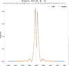Figure 2 The profile of the 002 reflection of TyrosineROD with 10 beams (blue). The integration step (orange) is adequate. Note that, due to dynamic interaction with neighbouring beams, the profile is split and wavy. The intensity profile obtained with the kinematic approximation would have a more Gaussian-like shape and would have its maximum intensity at . With this example, the intensity at is much smaller than the maximum intensity of this rocking curve.

3.3.1. Integration procedure

For each beam, the dynamical intensity profile I(S_g) is evaluated across a range of excitation errors around the ideal diffraction condition (). The final rocking curves are presented as a function of excitation error to clearly show how the reflection intensity changes as it passes through its ideal Bragg angle at .

Parametrizing the rocking curve in terms of S_g rather than rotation angle ω allows meaningful comparison between reflections: the rate at which S_g changes with ω depends on the distance of the reciprocal-lattice point from the rotation axis, so rocking curves plotted against ω have geometrically different widths for different reflections. In S_g space this geometric variation is removed, and the profile width reflects only the physical scattering properties of the reflection.

The integration proceeds as follows (see also Fig. 3):

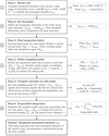Figure 3 Scheme 2. Dynamic reflection rocking-curve integration flowchart. Obtaining Idyn requires a full dynamic intensity profile calculation as a function of Sg [whereas Sg is a reciprocal-space dimension related to scan rotation angle ω, Sg(ω)].

(1) Broad scan: the profile is first computed over a wide range, typically  Å⁻¹, to identify the maximum intensity I_max.

(2) Threshold determination: a threshold intensity of is set to define the practical integration limits.

(3) Integration limits: starting from a broad S_g range, the profile is evaluated from both sides towards the centre in a first pass, during which the point at which the intensity rises above the intensity threshold is determined. The points at which this occurs define the integration interval .

(4) Sampling strategy: within the integration span, the profile is sampled at discrete points. The user specifies the number of integration points p on each side of , which determines the step size . To accurately capture the typically sharp peak near the ideal excitation condition, three additional points are included: one point at exactly and two points at . A good starting point for the number of integration points is (see Appendix B).

(5) Intensity calculation: for each sampling point, the structure matrix , the scattering matrix and parent beam intensity are recalculated for a given position as shown in Fig. 1.

(6) Numerical integration: the total dynamical intensity is obtained by trapezoidal integration of the sampled profile:

3.3.2. Implementation considerations

At each integration point, the structure matrix must be updated to reflect the changed excitation errors of all beams at that particular S_g value. This requires a new eigenvalue decomposition, construction of the scattering matrix and extraction of the parent beam intensity. Although this process involves multiple matrix operations per integration point, it remains computationally efficient when the number of coupled beams N is kept modest (typically 10–20).

The integration is performed in reciprocal space rather than in direct angular space. The Lorentz correction is applied during the CrysAlisPro data processing step. The Olex2 input hkl values have been corrected and are ready for refinement, as described in Section 2.1. This approach, analogous to the `Kabsch space' integration used in CrysAlisPro for X-ray data, ensures that dynamical profiles remain similar and independent of the reflection's position relative to the rotation axis. Integration in direct space would reproduce profiles whose widths vary with distance from the rotation centre.

3.3.3. Dependence on effective dynamical thickness

The width of the rocking-curve profile is strongly influenced by the effective dynamical thickness (EDT), which characterizes the strength of dynamical interactions in the crystal. Higher EDT values lead to narrower, more structured profiles with oscillations, requiring more integration points to accurately model the intensity. Conversely, a lower EDT produces broader, smoother profiles that can be adequately sampled with fewer points. The balance between integration accuracy and computational cost is controlled by the number-of-integration-points parameter, with typical values of 10–20 points per side yielding good results for EDT values up to 2000 Å.

3.4. Refinement

Refinement² begins by optimizing the EDT and batch-scale factors, using fixed coordinates and anisotropic parameters (ADPs). The starting model is the best kinematical model available, complete with anisotropic refinement and geometrically placed hydrogen atoms at neutron distances.

The number of N beams and the number of integration steps along the rotation axis control accuracy and speed; values of and 10 integration points provide a practical balance for typical electron diffraction data during the early stages of analysis.

After an approximate EDT has been determined (by refining it as the sole parameter), the other parameters – coordinates and ADPs – can now be included in the refinement, which will take significantly longer. If the sample is chiral, it is advisable to determine the absolute stereochemistry before adding additional parameters.

4. Absolute stereochemistry

Given adequate data quality, an advantage of electron diffraction over X-ray diffraction is the reliable determination of absolute stereochemistry in chiral materials, even for structures containing only light atoms where anomalous scattering is negligible.

4.1. Physical basis

In kinematical diffraction, Friedel's law states that reflections with indices hkl and have identical intensities, making it impossible to distinguish enantiomers. Multiple scattering breaks this symmetry: dynamical diffraction intensities depend on the phases of the structure factors, not just their magnitudes. Since inversion changes the sign of all structure-factor phases, the two enantiomers produce distinctly different dynamical intensity distributions.

Multi-beam interactions are required for this phase sensitivity to manifest. While three-beam methods can determine chirality in specific convergent-beam electron diffraction geometries (Johnson & Preston, 1994; Guo et al., 2018), in the context of integrated 3D-ED intensities the dominant contribution arises from four-beam and higher-order coupling (Spence et al., 1994), which ensures that Friedel-pair intensity differences are systematically present across the dataset rather than confined to specific orientations.

4.2. Determination procedure

The absolute stereochemistry cannot be determined directly from the diffraction data. Instead, both enantiomeric forms of the structure are refined independently using dynamical refinement, and their agreement with the observed data is compared. The enantiomer that yields better agreement (lower R factors, cleaner residual density) corresponds to the correct absolute configuration.

The N-Beam implementation uses the Z-score test (Klar et al., 2023) to quantify this comparison. The Z score quantifies the statistical significance of the difference in fit between the two enantiomers: a large positive Z score indicates that the current model is strongly favoured, whereas a large negative Z score suggests that the inverted structure is correct. In Olex2, this test is automatically run exactly once when N-Beam refinement is first enabled. This provides an early indication of the absolute stereochemistry of the molecule at hand – but for an accurate determination (especially in cases where the differences are small), more sophisticated built-in tools (full dynamic refinement of each hand) should be employed.

For high-quality electron diffraction data refined dynamically, Z scores often exceed 3, indicating very high confidence in the absolute configuration determination.

5. Non-spherical form factors

The N-Beam engine supports the NoSpherA2 approach (Kleemiss et al., 2021) for non-spherical atomic scattering factors, which accounts for aspherical electron density arising from chemical bonding, lone pairs and charge redistribution. This goes beyond the independent atom model (IAM) typically used in routine crystallography. The application of this approach in electron diffraction has a lot of potential, considering that the partial charges of atoms can be evaluated, and is subject to further research.

6. Validation using dynamical simulation

To verify the numerical consistency of the N-Beam implementation, a dedicated dynamical simulator was developed in CrysAlisPro.

Given an input crystal structure, UB orientation matrix and other parameters (N-Beam number, EDT, integration points etc.), the simulator calculates full dynamical intensities (hkl) based on the Bloch-wave formalism and generates synthetic diffraction frames.

These simulated frames can then be processed using CrysAlisPro in the same way as experimental data, yielding a processed reflection list suitable for N-Beam refinement in Olex2.

The validation test used an L-tyrosine model as input. Two datasets were compared: (i) the raw simulated integrated intensities and (ii) the intensities extracted from the simulated diffraction frames after standard CrysAlisPro processing.

When these datasets were `refined' in Olex2 using the initial input structural model (keeping all parameters fixed, except for the EDT), the resulting residuals were for the raw simulated intensities and for the automatically processed frame intensities (default settings). The EDT used in the simulation could also be recovered.

These results demonstrate that the N-Beam refinement reproduces the simulated dynamical intensities with near-perfect fidelity, confirming the implementation's internal consistency and compatibility with the CrysAlisPro data reduction pipeline.

7. Validation using a real L-tyrosine dataset

The performance of the N-Beam approach was evaluated using continuous-rotation electron diffraction data from an L-tyrosine crystal collected on a Rigaku Synergy-ED diffractometer.

Starting from a kinematical model (), refinement with produced a significant reduction in R values and correctly identified the absolute configuration.

The full set of files for this sample structure is packaged with Olex2. All diagnostic files generated for testing are included, and the test code used is available in Olex2.

The dependence of calculated rocking-curve profiles on the number of integration points p and EDT is presented in Fig. 6.

8. Availability

Olex2 is distributed as open-source software, whereas AutoChem and the N-Beam dynamical refinement extension are proprietary modules developed jointly with the Rigaku Corporation.

These are provided with Rigaku's CrysAlisPro-based X-ray and electron diffractometers. The integrated workflow is available to all CrysAlisPro users without additional software installation.

Data collected with a Rigaku Synergy-ED diffractometer are signed with a digest that enables the N-Beam dynamical refinement extension in Olex2 for each dataset on any computer. For electron diffraction data from other instruments, it is necessary to reduce and sign the data with CrysAlisPro, which requires a licence for both CrysAlisPro and AutoChem. The commercial licences can be obtained from the Rigaku Corporation.

9. Summary

The N-Beam implementation provides full dynamical refinement capabilities within the Olex2–CrysAlisPro environment.

By combining reliable data acquisition, automated model building and efficient Bloch-wave calculations, this workflow enables quantitative structure refinement and absolute structure determination from routine 3D electron diffraction data.

The approach makes dynamical refinement accessible to a broad community of crystallographers, providing a practical bridge between established X-ray practice and modern electron diffraction.

APPENDIX A

The N-Beam approach for dynamical refinement in Olex2

A1. Background: from Bloch wave to N-Beam

The N-Beam approach implemented in Olex2–AutoChem is based on the Bloch-wave formulation of electron diffraction (Hirsch et al., 1977; Colella, 1974).

Traditional implementations, such as those in Jana2006/Dyngo (Palatinus et al., 2013; Palatinus et al., 2015; Palatinus et al., 2019), evaluate these equations using a `virtual frame' approach. The rotation experiment is sliced by the data reduction program into virtual frames, which serve as a container for reflections in the region and carry a common group scale factor.

In contrast, N-Beam operates directly on the integrated reflection intensities exported by CrysAlisPro, modelling each reflection together with a selected local neighbourhood of interacting beams. The local neighbourhood can be set at refinement time in terms of interacting beams and grouping scale factors.

A2. Input data and model definition

Each reflection hkl is defined by its Bragg angle θ, scan limits , observed intensity and e.s.d. value.

The data reduction results in a single CIF containing all relevant information. Non-standard CIF items had to be defined because they did not yet exist.

_diffrn_frame_start_angle: details of the measurement registered frame where frame exposure started with the diffractometer being in this scanning angle position. For the Synergy-ED, the scanning angle is the grid tilt position.

_diffrn_frame_end_angle: details of the measurement registered frame where frame exposure ended with the diffractometer being in this scanning angle position. For the Synergy-ED, the scanning angle is the grid tilt position.

_diffrn_frame_scale: data processing output providing details of the final scale applied to intensities on a given frame.

_refln_frame_id: the experiment frame ID number where the given reflection has a central point.

_refln_diffraction_start_angle: data processing output providing details of where the given reflection integration profile starts within scanning angle space.

_refln_diffraction_end_angle: data processing output providing details of where the given reflection integration profile ends within scanning angle space.

_refln_intensity_scale_factor: data processing output providing details of the final scale applied to the intensity of a given reflection.

_diffrn_oxdiff_scatteringfactors_ed: reference to a table with atomic scattering factors used for all atoms. To be fully compliant with the International Union of Crystallography CIF dictionary, the per-atom definition using the entry _atom_type_scat_source should be used. We will update this inconsistency in future versions.

The reciprocal-space orientation matrix is supplied with other experimental data in CIF format. The initial structural model parameters are made by Olex2 standard kinematical approximation solution/refinement procedures.

A theoretical reflection list to a chosen resolution is generated to ensure continuity of beam neighbourhoods.

A3. Structure matrix

For each parent reflection, the coupling between the parent beam and its N neighbours is represented by the structure matrix . In a general N-Beam case,

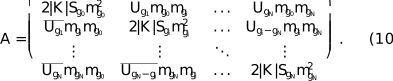
The dimensionality of is for a general N-Beam set. corresponds to the incident beam (000), the parent beam is and its neighbourhood beams are . The first element of the matrix () is equal to 0 as the length of the vector .

A4. Scattering matrix and beam propagation

The scattering matrix defines the propagation of coupled beams through the crystal:

t is EDT and is a diagonal matrix with elements m_gi as defined in equation (6). This exponential operator corresponds to Bloch-wave propagation, and the dynamical intensity of the parent beam is extracted from the second element of the first column of at each integration step. The first element is the 000 reflection; the set of calculated beams starts from the second matrix element: the parent beam with .

For the matrix exponential , where is a scalar and the matrix depends on a parameter q, assuming diagonalization of as in equation (11), the derivative with respect to the parameter q is given by (Tsai & Chan, 2003)

Here

and

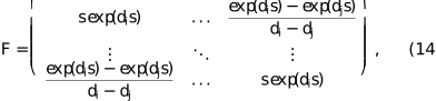
with d_i being the eigenvalues of and denoting the Hadamard product. The derivative of the matrix exponential by the scalar is identical to a normal exponential derivative.

APPENDIX B

Validation and testing

The N-Beam implementation was validated using three complementary approaches: (1) synthetic data with known ground truth to verify numerical accuracy, (2) synthetic data processed through the full experimental pipeline to test software integration and (3) real experimental data to demonstrate practical performance. All three tests used L-tyrosine as the model system (Fig. 4).

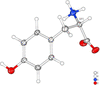Figure 4 Displacement parameter diagram of a real structure of tyrosine, tyrosineED (IAM).

B1. Test datasets

B1.1. TyrosineRAW: numerical consistency test

The TyrosineRAW dataset consists of dynamical intensities computed directly from a known L-tyrosine structure using the same Bloch-wave formalism implemented in N-Beam. The simulator (described in Section 6) generated reflection intensities based on specified structural parameters (atomic positions, displacement parameters, EDT) and N-Beam settings set to N = 20 and p = 40 (integration points). These raw synthetic intensities were then imported into Olex2 and `refined' against the original structural model with all parameters held fixed except EDT.

This test isolates numerical accuracy: any discrepancy between calculated and `observed' intensities reveals implementation errors, rounding issues or algorithmic inconsistencies. The resulting agreement was , and the input EDT (300 Å) was recovered exactly. This near-perfect agreement confirms the internal consistency of the N-Beam calculations.

B1.2. TyrosineCAP: pipeline integration test

The TyrosineCAP dataset tests the complete data processing workflow. The same synthetic dynamical intensities from TyrosineRAW were used to generate simulated diffraction frames – pixelated detector images mimicking a real rotation experiment. These frames were then processed through the full CrysAlisPro integration pipeline (profile fitting, background subtraction, Lorentz correction etc.) to produce a reflection list with integrated intensities and experimental metadata.

This processed reflection list was refined in Olex2 using N-Beam, again with all structural parameters fixed except EDT. The resulting is slightly higher than that for TyrosineRAW due to small systematic effects introduced by the integration procedure (binning, profile fitting, numerical precision in the frame-to-reflection transformation). EDT was again recovered correctly.

This test confirms that the N-Beam engine correctly interprets the extended CIF format exported by CrysAlisPro, properly reconstructs the measurement geometry for each reflection and produces results compatible with the integration software's conventions.

B1.3. TyrosineED: real experimental data

The TyrosineED dataset consists of continuous-rotation electron diffraction data collected from a real L-tyrosine crystal on a Rigaku Synergy-ED diffractometer. Starting from a kinematical refinement with , dynamical refinement with beams reduced R₁ to approximately 8%. The absolute configuration was correctly determined with high confidence (Z =). At these settings, a refinement cycle (full refinement) will take seconds. With , the final R₁ was 6.86% with a Z score of 18.7 and an R₁ difference of 6.07% (see Table 1).

Table 1
Crystallographic data for TyrosineED

Compound	TyrosineED
Formula	C9H11NO3
Dcalc (g cm^−3)	1.381
μ (mm^−1)	0.000
Formula weight (g mol^−1)	181.191
Colour	Colourless
T (K)	293
Crystal system	Orthorhombic
Space group	P212121
a (Å)	5.8600 (4)
b (Å)	6.9913 (13)
c (Å)	21.2698 (15)
α (°)	90
β (°)	90
γ (°)	90
V (Å^3)	871.40 (18)
Z	4
	1
Wavelength (Å)	0.02510
Radiation type	Electron
(°)	0.12
(°)	0.90
Index range h
Index range k
Index range l
Measured reflections	3269
Independent reflections	3269
Reflections.	2640
	0.0868
Parameters	186
Restraints	192
Largest peak (e Å^−1)	0.1630
Deepest hole (e Å^−1)	−0.2116
Goodness of fit	1.270
R1 [ / all]	0.0686 / 0.0759
wR2 [ / all]	0.1760 / 0.1815
Z score	18.70
	6.07
N-Beam settings
N-Beams	30
Integration points	30
Float	True

This result demonstrates that the N-Beam approach achieves the expected improvement over kinematical refinement for real experimental data, where imperfections in crystal quality, detector response, beam coherence and other factors introduce noise absent from the synthetic datasets.

B2. Comparison of datasets

Fig. 5 shows versus plots for all three datasets. The TyrosineRAW data [Fig. 5(a)] lie almost perfectly on the diagonal, confirming numerical fidelity. TyrosineCAP [Fig. 5(b)] shows slightly increased scatter due to integration artefacts, but the correlation remains excellent. TyrosineED [Fig. 5(c)] exhibits broader scatter characteristic of real experimental data, but the overall correlation is strong and systematic deviations are absent, indicating that dynamical effects are being correctly modelled.

Figure 5 Observed versus calculated intensity plots for the three L-tyrosine test datasets. (a) TyrosineRAW: synthetic data refined against the generating model, . (b) TyrosineCAP: synthetic data processed through CrysAlisPro integration, . (c) TyrosineED: real experimental data, after dynamical refinement (IAM).

B3. Optimization of beam number

A key practical question is how many beams N are necessary for accurate dynamical refinement? Using too few beams underestimates intensity redistribution; using too many increases computation time without improving results.

Fig. 6 shows the dependence of R₁ and Z score on the number of beams for the TyrosineED dataset. Both metrics stabilize at 12–15: further increases in N produce negligible changes in fit quality or absolute structure determination. This convergence behaviour was observed consistently across multiple test structures.

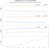Figure 6 Convergence of refinement quality with increasing beam number for TyrosineED. R1, wR2 and the absolute structure Z score all plateau beyond 12–15, indicating that a moderate number of beams is sufficient for all practical purposes. The absolute stereochemistry can be reliably established even with very few beams. Spherical form factors were used.

The optimal beam number depends weakly on crystal thickness (EDT) and diffraction geometry, but 10–20 provides a good balance between accuracy and speed for typical electron diffraction datasets. Users can verify convergence by performing trial refinements with varying N and checking for stability in R factors and refined parameters.

B4. Computational performance

Refinement time scales approximately as N^2.8 due to the eigenvalue decomposition of the structure matrix at each integration point. For N = 10 and 10 integration points per side, a typical dataset of 500–1000 reflections refines in 12 s (full refinement of tyrosine, 4 least-squares cycles) on a standard office laptop (Intel i7-865U @ 1.90GHz, 4 cores). Increasing N and p to 20 extends this to 90 s, and even going to n = p = 40 will take less than 5 min, which remains practical for routine use.

Profile integration sampling (10–20 points per side) adequately reproduces rocking-curve shapes for EDT values up to ∼2000 Å, which covers most small-molecule electron diffraction applications. A higher EDT or more complex dynamical behaviour may require denser sampling or adaptive integration strategies.

B5. Summary of validation results

The three-tier validation strategy demonstrates:

(i) Numerical accuracy: TyrosineRAW confirms that the Bloch-wave calculations are implemented correctly ().

(ii) Pipeline integration: TyrosineCAP verifies compatibility with CrysAlisPro data processing ().

(iii) Real-world performance: TyrosineED shows the expected improvement from kinematical to dynamical refinement on experimental data ( R₁: 15% ∼7%).

The beam-number convergence test shows that 12–15 is sufficient for most applications, and computational performance is acceptable for routine structural work. These results confirm that N-Beam is both scientifically rigorous and practically viable for everyday crystallographic analysis.

APPENDIX C

Notation

n (vector, magenta) (Fig. 7): unit vector normal to the crystal entrance surface, directed away from the crystal towards the electron source. Fixed in the laboratory frame; the crystal rotates relative to it via the rotation matrix R(ω) applied to the orientation matrix UB.

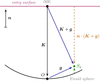Figure 7 Geometry of the Ewald sphere construction and the notation used in this text. Solid arrows, vectors; dashed arrows, scalars. Bold symbols follow the notation of the main text.

K (vector, black): electron wavevector inside the crystal, from the centre of the Ewald sphere to the origin O of reciprocal space (the 000 beam). Its magnitude |K| differs slightly from the electron wavevector in vacuum due to the mean inner potential of the crystal. The scalar is the projection of K onto the surface normal; since K and n are antiparallel, K_n is negative and . K_n enters the obliquity correction factors m_gi (see the main text) and the scattering matrix exponent .

g (vector, blue): reciprocal-lattice vector of the reflection under consideration, pointing from the origin O to the reciprocal-lattice point G.

K + g (vector, blue): diffracted beam wavevector, from the centre of the Ewald sphere towards the reciprocal-lattice point G. When G lies exactly on the Ewald sphere, |K + g| = |K| and the Bragg condition is exactly satisfied (S_g = 0).

S_g (scalar, green): deviation parameter (excitation error), the signed distance from the reciprocal lattice point G to the Ewald sphere, measured along n. As used in the main text:

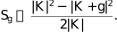
The exact form from the diagram geometry is

When S_g = 0 the Bragg condition is exactly satisfied; reflections with small |S_g| still contribute due to the finite crystal thickness.

(scalar, orange): projection of (K + g) onto n. The perpendicular distance from the entrance surface to the reciprocal-lattice point G along n; enters the exact expression for S_g above.

Supporting information

Computing details

(I)

Crystal data

C9H11NO3	Z = 4
Mr = 181.19	F(000) = 146.196
Orthorhombic, P212121	Dx = 1.381 Mg m^−3
a = 5.8600 (4) Å	Electron radiation, λ = 0.02510 Å
b = 6.9913 (13) Å	Cell parameters from 2400 reflections
c = 21.2698 (15) Å	θ = 0.1–0.9°
V = 871.40 (18) Å^3	µ = 0.00 mm^−1

Data collection

XtaLAB Synergy-ED, HyPix-ED, electron source at 200keV diffractometer	3269 independent reflections
Radiation source: electron diffractometer, JEOL JSM-2300ED, LaB6	2640 reflections with I ≥ 2u(I)
None monochromator	Rint = 0.087
Detector resolution: 10.0000 pixels mm^-1	θmax = 0.9°, θmin = 0.1°
continuous rotation electron diffraction scans	h = −7→7
Absorption correction: multi-scan CrysAlisPro 1.171.44.75a (Rigaku Oxford Diffraction, 2024) Empirical absorption correction using spherical harmonics, implemented in SCALE3 ABSPACK scaling algorithm.	k = −7→7
Tmin = 0.746, Tmax = 1.000	l = −26→26
3269 measured reflections

Refinement

Refinement on F^2	120 parameters
Least-squares matrix: full	0 restraints
R[F^2 > 2σ(F^2)] = 0.069	19 constraints
wR(F^2) = 0.182	H-atom parameters constrained
S = 1.27	w = 1/[σ^2(Fo^2) + (0.070P)^2] where P = (Fo^2 + 2Fc^2)/3
1476 reflections	(Δ/σ)max = 0.009

Fractional atomic coordinates and isotropic or equivalent isotropic displacement parameters (Ų)

	x	y	z	Uiso*/Ueq
O10	0.3727 (4)	0.8312 (7)	0.33256 (12)	0.0394 (12)
O11	0.2311 (4)	0.5709 (7)	0.28583 (11)	0.0374 (11)
O13	0.5307 (4)	0.5183 (6)	0.59918 (9)	0.0346 (10)
H13	0.6659 (16)	0.569 (3)	0.62073 (18)	0.0519 (15)*
N	0.8041 (4)	0.7580 (6)	0.30452 (11)	0.0335 (10)
Ha	0.7766 (11)	0.8659 (8)	0.2720 (3)	0.0403 (12)*
Hb	0.7829 (11)	0.8119 (11)	0.3495 (2)	0.0403 (12)*
Hc	0.9686 (4)	0.7059 (6)	0.2996 (4)	0.0403 (12)*
C1	0.6466 (4)	0.4595 (7)	0.40552 (11)	0.0241 (11)
C2	0.4388 (4)	0.4057 (7)	0.43328 (11)	0.0290 (11)
H2	0.3044 (4)	0.3476 (7)	0.40402 (11)	0.0348 (13)*
C3	0.4017 (5)	0.4257 (8)	0.49799 (11)	0.0334 (12)
H3	0.2420 (5)	0.3792 (8)	0.51853 (11)	0.0401 (14)*
C4	0.5728 (4)	0.5065 (7)	0.53640 (11)	0.0244 (11)
C5	0.7766 (4)	0.5684 (7)	0.50896 (11)	0.0313 (11)
H5	0.9055 (4)	0.6370 (7)	0.53764 (11)	0.0376 (13)*
C6	0.8148 (4)	0.5421 (7)	0.44453 (11)	0.0313 (11)
H6	0.9762 (4)	0.5857 (7)	0.42429 (11)	0.0376 (14)*
C7	0.6896 (5)	0.4285 (7)	0.33604 (11)	0.0341 (11)
H7a	0.5883 (5)	0.3078 (7)	0.32067 (11)	0.0409 (13)*
H7b	0.8672 (5)	0.3907 (7)	0.32976 (11)	0.0409 (13)*
C8	0.6358 (4)	0.5986 (7)	0.29358 (10)	0.0270 (11)
H8	0.6492 (4)	0.5522 (7)	0.24440 (10)	0.0324 (13)*
C9	0.3915 (5)	0.6752 (7)	0.30506 (12)	0.0277 (12)

Atomic displacement parameters (Ų)

	U^11	U^22	U^33	U^12	U^13	U^23
O10	0.0298 (12)	0.048 (4)	0.0401 (13)	0.0067 (18)	0.0067 (11)	−0.0010 (16)
O11	0.0210 (10)	0.048 (3)	0.0430 (12)	−0.0042 (17)	−0.0023 (9)	−0.0040 (15)
O13	0.0307 (11)	0.044 (3)	0.0294 (11)	−0.0017 (16)	−0.0004 (9)	−0.0044 (14)
N	0.0224 (11)	0.052 (3)	0.0259 (11)	0.0020 (16)	0.0003 (9)	−0.0039 (14)
C1	0.0188 (12)	0.030 (4)	0.0239 (12)	−0.0006 (18)	−0.0021 (9)	−0.0019 (14)
C2	0.0205 (12)	0.042 (4)	0.0244 (13)	−0.0069 (19)	−0.0026 (10)	0.0003 (16)
C3	0.0225 (12)	0.052 (4)	0.0255 (13)	−0.009 (2)	0.0004 (10)	−0.0012 (16)
C4	0.0177 (11)	0.029 (4)	0.0266 (12)	−0.0021 (18)	−0.0003 (10)	−0.0001 (14)
C5	0.0218 (12)	0.047 (4)	0.0253 (12)	−0.0014 (19)	−0.0021 (10)	−0.0041 (16)
C6	0.0179 (11)	0.050 (4)	0.0265 (12)	−0.0056 (19)	−0.0027 (10)	0.0030 (16)
C7	0.0271 (12)	0.047 (4)	0.0280 (13)	0.010 (2)	0.0020 (11)	−0.0047 (17)
C8	0.0206 (12)	0.041 (4)	0.0195 (11)	0.0013 (19)	0.0017 (10)	−0.0004 (14)
C9	0.0171 (13)	0.042 (4)	0.0238 (12)	0.0013 (18)	0.0025 (10)	−0.0041 (16)

Geometric parameters (Å, º)

O10—C9	1.242 (6)	C2—C3	1.400 (3)
O11—C9	1.258 (5)	C3—C4	1.411 (4)
O13—C4	1.360 (3)	C4—C5	1.398 (4)
N—C8	1.507 (5)	C5—C6	1.401 (3)
C1—C2	1.404 (4)	C7—C8	1.526 (6)
C1—C6	1.412 (4)	C8—C9	1.548 (4)
C1—C7	1.515 (3)
C6—C1—C2	117.9 (2)	C5—C6—C1	121.1 (3)
C7—C1—C2	121.1 (3)	C8—C7—C1	115.5 (3)
C7—C1—C6	121.1 (2)	C7—C8—N	110.5 (2)
C3—C2—C1	121.4 (3)	C9—C8—N	109.0 (3)
C4—C3—C2	119.9 (3)	C9—C8—C7	111.6 (2)
C3—C4—O13	117.6 (2)	O11—C9—O10	126.6 (3)
C5—C4—O13	123.1 (3)	C8—C9—O10	117.4 (3)
C5—C4—C3	119.3 (2)	C8—C9—O11	116.0 (4)
C6—C5—C4	120.3 (3)

 

Footnotes

¹Residual density maps are computed as described on p. 7 of the appendix of Palatinus et al. (2017) and are further scaled (in order to convert Å⁻² into e Å⁻¹ units of the electrostatic potential) according to the method of Gruza et al. (2020).

²Details of the structure-factor calculations are provided in Appendix A (Sections A3 and A4). If an extinction parameter is present in the instructions, it will be ignored.

References

Allen, F. H. & Bruno, I. J. (2010). Acta Cryst. B66, 380–386. Web of Science CrossRef CAS IUCr Journals Google Scholar
Beanland, R., Evans, K., Römer, R. A. & Hubert, A. J. M. (2019). Felix, https://github.com/WarwickMicroscopy/Felix. Google Scholar
Bethe, H. A. (1928). Annalen Phys. 392, 55–129. CrossRef Google Scholar
Bourhis, L. J., Dolomanov, O. V., Gildea, R. J., Howard, J. A. K. & Puschmann, H. (2015). Acta Cryst. A71, 59–75. Web of Science CrossRef IUCr Journals Google Scholar
Brázda, P., Palatinus, L. & Babor, M. (2019). Science 364, 667–669. Web of Science PubMed Google Scholar
Cleverley, A. & Beanland, R. (2022). Acta Cryst. A78, e625. CrossRef IUCr Journals Google Scholar
Cleverley, A. & Beanland, R. (2023). IUCrJ 10, 118–130. CrossRef CAS PubMed IUCr Journals Google Scholar
Colella, R. (1974). Acta Cryst. A30, 413–423. CrossRef CAS IUCr Journals Web of Science Google Scholar
Dolomanov, O. V., Bourhis, L. J., Gildea, R. J., Howard, J. A. K. & Puschmann, H. (2009). J. Appl. Cryst. 42, 339–341. Web of Science CrossRef CAS IUCr Journals Google Scholar
Gruza, B., Chodkiewicz, M. L., Krzeszczakowska, J. & Dominiak, P. M. (2020). Acta Cryst. A76, 92–109. Web of Science CrossRef IUCr Journals Google Scholar
Guo, Y., Nakashima, P. N. H. & Etheridge, J. (2018). IUCrJ 5, 753–764. CrossRef CAS PubMed IUCr Journals Google Scholar
Hirsch, P., Howie, A., Nicholson, R., Pashley, D. & Whelan, M. (1977). Electron Microscopy of Thin Crystals. Robert E. Krieger Publishing Company. Google Scholar
Ito, S., White, F. J., Okunishi, E., Aoyama, Y., Yamano, A., Sato, H., Ferrara, J. D., Jasnowski, M. & Meyer, M. (2021). CrystEngComm 23, 8622–8630. Web of Science CSD CrossRef CAS Google Scholar
Johnson, A. W. S. & Preston, A. R. (1994). Ultramicroscopy 55, 348–355. CrossRef CAS Google Scholar
Kabsch, W. (1988). J. Appl. Cryst. 21, 67–72. CrossRef CAS Web of Science IUCr Journals Google Scholar
Kabsch, W. (2010a). Acta Cryst. D66, 125–132. Web of Science CrossRef CAS IUCr Journals Google Scholar
Kabsch, W. (2010b). Acta Cryst. D66, 133–144. Web of Science CrossRef CAS IUCr Journals Google Scholar
Klar, P. B., Krysiak, Y., Xu, H., Steciuk, G., Cho, J., Zou, X. & Palatinus, L. (2023). Nat. Chem. 15, 848–855. Web of Science CSD CrossRef CAS PubMed Google Scholar
Kleemiss, F., Dolomanov, O. V., Bodensteiner, M., Peyerimhoff, N., Midgley, A., Bourhis, L. J., Genoni, A., Malaspina, L. A., Jayatilaka, D., Spencer, J. L., White, F., Grundkötter-Stock, B., Steinhauer, S., Lentz, D., Puschmann, H. & Grabowsky, S. (2021). Chem. Sci. 12, 1675–1692. CrossRef CAS Google Scholar
Matsumoto, T., Yamano, A., Sato, T., Ferrara, J. D., White, F. J. & Meyer, M. (2021). J. Chem. Crystallogr. 51, 438–450. Web of Science CSD CrossRef CAS Google Scholar
Palatinus, L., Brázda, P., Boullay, P., Perez, O., Klementová, M., Petit, S., Eigner, V., Zaarour, M. & Mintova, S. (2017). Science 355, 166–169. Web of Science CSD CrossRef ICSD CAS PubMed Google Scholar
Palatinus, L., Brázda, P., Jelínek, M., Hrdá, J., Steciuk, G. & Klementová, M. (2019). Acta Cryst. B75, 512–522. Web of Science CrossRef IUCr Journals Google Scholar
Palatinus, L., Corrêa, C. A., Steciuk, G., Jacob, D., Roussel, P., Boullay, P., Klementová, M., Gemmi, M., Kopeček, J., Domeneghetti, M. C., Cámara, F. & Petříček, V. (2015). Acta Cryst. B71, 740–751. Web of Science CrossRef IUCr Journals Google Scholar
Palatinus, L., Jacob, D., Cuvillier, P., Klementová, M., Sinkler, W. & Marks, L. D. (2013). Acta Cryst. A69, 171–188. Web of Science CrossRef CAS IUCr Journals Google Scholar
Palatinus, L., Petříček, V. & Corrêa, C. A. (2015). Acta Cryst. A71, 235–244. Web of Science CrossRef IUCr Journals Google Scholar
Peng, L. (1999). Micron 30, 625–648. CrossRef CAS Google Scholar
Seto, Y. & Ohtsuka, M. (2022). J. Appl. Cryst. 55, 397–410. Web of Science CrossRef CAS IUCr Journals Google Scholar
Spence, J. C. H., Zuo, J. M., O'Keeffe, M., Marthinsen, K. & Hoier, R. (1994). Acta Cryst. A50, 647–650. CrossRef CAS Web of Science IUCr Journals Google Scholar
Tsai, H. & Chan, K. S. (2003). Bernoulli 9, 895–919. CrossRef Google Scholar
Zuo, J. M. & Weickenmeier, A. L. (1995). Ultramicroscopy 57, 375–383. CrossRef CAS Google Scholar
Zou, X., Hovmöller, S. & Oleynikov, P. (2011). Electron Crystallography. International Union of Crystallography Texts on Crystallography, 16. Oxford University Press. Google Scholar
This is an open-access article distributed under the terms of the Creative Commons Attribution (CC-BY) Licence, which permits unrestricted use, distribution, and reproduction in any medium, provided the original authors and source are cited.