

 menu


research papers
 | JOURNAL OF APPLIED CRYSTALLOGRAPHY |
 access
A JUNGFRAU-based electron diffractometer with large-scale capacity

aInstitute of Inorganic Chemistry, University of Vienna, Vienna, Austria, and bPaul-Scherrer-Institut, Villigen, Switzerland
*Correspondence e-mail: [email protected]
An integrated hardware–software platform for three-dimensional electron diffraction has been developed using the JUNGFRAU 1M charge-integrating hybrid pixel detector. The system combines the field-programmable gate array based Jungfraujoch backend with the JFGui graphical interface, providing centralized control of the detector, electron microscope and data-processing software. This workflow enables synchronized data acquisition, live visualization and instantaneous post-processing with established crystallographic programs, including XDS, DIALS and SHELX. Applications to L-histidine and dioctyl perylene tetracarboxylic diimide crystals are presented, including charge-density evaluation employing the recently developed iSFAC (ionic scattering factors) model. The workflow supports continuous-rotation measurements at speeds up to 10° s−1, allowing acquisition of a ∼130° rotation in approximately 15 s and enabling higher-throughput measurements. Comparative measurement at 100 and 200 keV beam energies revealed the trade-off between real-space contrast and diffraction resolution. These developments establish a complete and efficient practical workflow of 3D ED coupled with instrumental evaluation, providing a robust route toward quantitative electron crystallography.
1. Introduction
Structure determination using three-dimensional electron diffraction (3D ED) has emerged as a powerful technique over the past 15 years. Owing to its applicability to sub-micrometre-sized crystals, it has enabled the elucidation of structures across diverse fields of chemistry. Continuous developments in methodology and instrumentation have further expanded its capabilities, resulting in several variants of 3D ED techniques (Smeets et al., 2018 ; Gemmi et al., 2019; Yörük et al., 2024). Another notable advantage of 3D ED lies in the higher sensitivity of electron scattering to charge density compared with X-ray diffraction (Zuo et al., 1999; Yonekura et al., 2018; Takaba et al., 2023). Pioneering studies have demonstrated its potential for experimental evaluation of charge distribution within molecules, highlighting a unique strength of electron-based approaches (Suresh et al., 2024; Pacoste et al., 2024; Mahmoudi et al., 2025). Despite these advantages, 3D ED has not yet become a mainstream method for structure determination. The Cambridge Structural Database [Cambridge Crystallographic Data Center (CCDC)] (Groom et al. (2016) lists 239 entries in the electron diffraction subset for the period 2022–2024, corresponding to 0.140% of all new entries. Even when accounting for limited instrument availability, this indicates that 3D ED remains far from being a first-choice technique, despite the less stringent requirements for crystal growth compared with X-ray diffraction. Currently, 3D ED and its advanced applications still require more time and effort than conventional methods. Unless these limitations are addressed, the broader impact of 3D ED and the structural insights that can be provided to chemistry, e.g. drug design, materials science and charge-density analysis, will remain constrained.
In 3D ED, a diffraction volume can be collected from a single crystal on a transmission electron microscope (TEM) grid with continuous stage rotation. However, in application to organic chemistry, limited lattice symmetry, variations in crystallinity and heterogeneity in crystal grain morphologies often necessitate collection of multiple datasets and their merging. Several software packages have been developed to enable sequential data collection, including SerialEM (Mastronarde, 2005; de la Cruz et al., 2019; Takaba et al., 2020; Sasaki et al., 2023), Instamatic (Wang et al., 2019; Roslova et al., 2020), EPU-D (Thermo Fisher Scientific) and CrysAlisPro for ED (Rigaku) (Ito et al., 2021). Considering the instability of the electron beam on events inducing fluctuations, it is appropriate to collect diffraction datasets from multiple crystals maintaining the beam condition unchanged. This is particularly true for active-pixel sensor detectors, where changes in beam conditions risk detector damage from unexpected direct-beam incidence. Consequently, a uniform exposure rate is usually adopted. In addition, to account for the lower dose tolerance of crystals of smaller volume sampled across a collection sequence, a reduced exposure rate tends to be preferred. An exposure of ∼1 e− Å−2 per single rotation is often selected, following the applications for macromolecules, which are the most beam-sensitive targets of 3D ED (Gruene et al., 2018; Ito et al., 2021; Martynowycz et al., 2022). Although this strategy is reasonable for samples containing limited types of elements and structural motifs, the optimal irradiation conditions should depend on sample composition and the target precision: heavier elements and aromatic systems may tolerate higher doses (Egerton, 2019), whereas higher-precision studies require reduced exposure (Howells et al., 2009).
Hybrid pixel detectors allow beam conditions to be changed without special consideration for TEM operation thanks to their radiation hardness, with which even direct-beam irradiation is feasible. The JUNGFRAU is a charge-integrating hybrid pixel detector initially developed for X-ray free-electron lasers (XFELs) and synchrotron applications (Mozzanica et al., 2016; Leonarski et al., 2018). Similarly to other hybrid pixel detectors, such as Timepix (Genderen et al., 2016), EIGER (Tinti et al., 2018) and SINGLA (Parkhurst et al., 2023), its application to electron diffraction has been proposed (Fröjdh et al., 2020). Compared with these counting detectors, JUNGFRAU offers a linear response over a wider dynamic range (Leonarski et al., 2018; Fröjdh et al., 2024). The in-pixel gain switching provides a dynamic range of 120 MeV px−1 frame−1 with 2 kHz frame rate, which corresponds to  e− px−1 s−1 for 200 kV electrons. Accurate measurement of both intense and weak diffraction spots is particularly important when aiming to quantify charge distribution in crystals, since photons and electrons scatter differently from core and valence charge over a broad scattering angle range.
To harness these advantages for practical 3D ED, an integrated hardware–software system is essential for end-users to conduct data collection efficiently. A field-programmable gate array (FPGA)-based backend, Jungfraujoch, has been developed as a control and readout system for data acquisition at synchrotron beamlines with JUNGFRAU, operating at 2 kHz (Leonarski et al., 2023). Building on this, we developed an integrated framework that couples JUNGFRAU and Jungfraujoch to a JEOL electron microscope via a user interface, JFGui (Ferjaoui et al., 2025). Following the initial demonstration of the detector platform, successive developments have transformed JFGui into an integrated environment for routine 3D ED measurements. In addition to the synchronization between data acquisition and crystal rotation, the current implementation incorporates live visualization, calibration in both real and reciprocal space, and integrated post-processing, allowing users to perform all essential experimental operations within a single interface. Thus, insights into sample properties can be obtained at the earliest measurement stages, allowing beam conditions to be adaptively tuned. The system is designed with extensibility in mind, between the JUNGFRAU and the modern electron microscopy setups.
In the following sections we introduce the EPOC (Electrostatic Potential of Compounds) software suite, focusing on its function for 3D ED. We then demonstrate its capabilities on cases for organic samples. Applications of the simplest charge-density analysis, iSFAC (ionic scattering factors), which we recently proposed (Mahmoudi et al., 2025), are presented as an aim of the workflow. Exploiting the features of JUNGFRAU aligned with the developed software, the feasibility and efficiency of high-speed rotation measurement and lower-energy beams are verified to elucidate the performance and limitations of the current instrument.
2. Materials and methods
2.1. Sample preparation
Crystals of L-histidine (Fluka) were taken directly from the bottle and suspended in n-hexane. The suspension was sonicated to crush and disperse the crystalline grains. Dioctyl perylene tetracarboxylic diimide (PTCDI-C8) nanowires were prepared following the reported procedure (Briseno et al., 2007); thin red crystals were precipitated from methanol. Perylene powder (FUJIFILM Wako) was dissolved in acetone, and the solution was injected into vigorously stirred water using a Hamilton syringe injector, resulting in the immediate formation of crystalline grains (Li et al., 2019). For all samples, a few microlitres of the suspension were dropped onto a copper grid coated with a lacey-carbon film and air-dried for several minutes. Each grid was inserted into the column of the electron microscope using a single-tilt cryo-sample holder, Gatan Elsa Model 698 (GATAN). The operating room temperature was maintained at 22°C, and the sample temperature control of the holder was used only for cryo-measurements.
2.2. Hardware and software framework
2.2.1. System overview
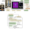
The hardware architecture and the basic workflow for single-rotation collection have been described previously (Ferjaoui et al., 2025). In summary, the JUNGFRAU 1M detector was mounted on a JEOL JEM2100Plus transmission electron microscope. The projected images on the detector are acquired through a Linux server running the FPGA-accelerated framework Jungfraujoch (Leonarski et al., 2023). Jungfraujoch manages measurement control (start/stop/cancel) through the jfjoch_broker and saves images via the jfjoch_writer. The microscope is operated using its console and PyJEM, the Python-based interface, version 3.8 (JEOL, 2018). All components communicate through JFGui, a Qt-based graphical user interface developed for this setup and derived from SinglaGUI (Maisriml & Gruene, 2024). JFGui runs on a dedicated Linux workstation to avoid resource contention during image acquisition. It communicates with the microscope PC via a relay script, simple-tem, which wraps the PyJEM API and exposes a small command interface used by JFGui to send control commands and receive real-time status updates from the TEM.
Communication between Jungfraujoch and JFGui is managed by a wrapper from epoc-utils, ensuring synchronization between user control and acquisition servers. Status values (e.g. lens conditions, stage position, camera settings) are saved as metadata within an HDF5 master file alongside image frames. A Python utility, metadata-updater, handles this information for later use during post-processing by the PostprocessServer_JFED. A separate CCDCscreener script queries crystal information from the CCDC. ShelXFile_EDiSFAC, an extension of the SHELXL (Sheldrick, 2015a) parser ShelXFile (Kratzert, 2018), allows quick application of the iSFAC modeling and its visualization for evaluation of atomic charge distributions (Mahmoudi et al., 2025). Fig. 1 illustrates the interconnections between these software components and the structure of the resulting HDF5 output.
|
Figure 1
Hardware and software configuration. (a) Central role of JFGui in coordinating communication between hardware and software components. (b) Representative metadata structure stored within the HDF5 output file; only major tags are shown. |
2.2.2. Live visualization
JFGui receives the live image stream from Jungfraujoch, processed on the FPGA where frame summation is performed before transmission. Users can toggle between automatic and preset contrast settings to visualize both real-space and diffraction images. In LowMAG mode, images are downsampled and arranged into a grid atlas. Beam intensity is estimated from the modal pixel value corresponding to the open-grid area. JFGui reports electron dose as intensity scaled by the illuminated area, expressed in Å−2 s−1. In DIFF mode, the software quantifies beam shape from peak height and width, identifies the beam center, and uses this for FPGA-based spot finding. Detected spot properties are sent back to JFGui to estimate diffraction resolution. These spots are also referenced to assess elliptical distortion in the calibration mode (see Section 2.2.3). Combining spot coordinates with the stage tilt allows visualization of the diffraction pattern in 3D reciprocal space. These visualization features operate at  20 frames per second, enabling fully interactive, real-time feedback during data collection.
2.2.3. Calibration
Magnification calibration in both real and reciprocal space is handled through lookup tables (LUTs) that map nominal to measured values. Real-space magnification is determined using a grating grid (TED PELLA). In reciprocal space, the magnification can be termed camera length, which depends not only on the nominal value but also on other parameters constructing the beam path, such as the operating accelerating voltage, probe size and any other conditions that can vary due to the hysteresis of electromagnetic lenses. The current implementation interpolates the determined values sampled across three major parameters: accelerating voltage, magnification and nominal camera length. The LUT is constructed from Debye–Scherrer ring measurements of an evaporated aluminium standard grid (Agar Scientific) under various configurations. Standard distances are obtained by azimuthal integration of diffraction patterns, with corrections for elliptical distortion. Because JUNGFRAU tolerates direct-beam incidence, JFGui performs a parallel, real-time 2D Gaussian fit within a region of interest (ROI) around the direct beam, using only non-saturated pixels, to extract the amplitude, centroid
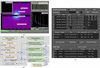
(x0,y0), widths  and tilt θ, which are continuously displayed to guide focus adjustment (Ferjaoui et al., 2025). In calibration mode, both the 1D intensity profile and the calculated camera length are displayed to verify ring positions against expected values. All calibration data and microscope parameters are stored in a JSON file, referenced throughout subsequent sessions. Fig. 2(a) represents this functionality and Movie 1 in the supporting information demonstrates a typical calibration measurement workflow.
|
Figure 2
JFGui features and data-processing workflow. (a) Calibration measurement interface showing beam and magnification evaluation; labels with gray background are external annotations. A guide rectangle is used for centering between LowMAG and MAG modes. (b) Flow chart summarizing the data-collection and processing workflow; gray-shaded steps are directly controllable through the GUI. (c) Representative display of multiple datasets collected and merged. Results from XDS and DIALS appear in paired rows of the top table. After several datasets have been collected, data-merging can start, and the output is shown in the middle table. If CCDC depositions with similar lattice parameters to the determined ones are identified, they are listed in the bottom table. The matches in the ELECTRON subset are checked. |
2.2.4. Diffraction data collection and post-processing
Crystals for diffraction measurements are first identified in LowMAG mode (typically ×1200 magnification) and centered manually or by directly clicking the position within JFGui. The stage height is adjusted to maintain eucentricity, first coarsely in LowMAG and then precisely in MAG mode. After switching to DIFF mode, data collection proceeds with synchronized control of continuous stage rotation. Buffered frames are stored in a NeXus-compliant HDF5 file by jfjoch_writer, and metadata-updater appends microscope parameters (accelerating voltage, lens currents, aperture size and position, and stage coordinates), following the EMD format of electron microscopy (Savitzky, 2023) [Fig. 1(b)]. To secure the experimental data as self-contained for downstream analysis, each dataset stores the direct beam position, estimated dose, calibrated camera length, rotation axis and stage tilt-angle readout list during continuous rotation. The spot-plotter module provides a live 3D visualization of detected diffraction spots. Post-processing via PostprocessServer_JFED includes background subtraction, 3D spot finding and indexing with XDS (Kabsch, 2010b) supported by the Dectris Neggia plugin (Dectris, 2017), and optionally with DIALS (Winter et al., 2018). Upon successful indexing, lattice parameters and crystal orientations are displayed in JFGui. The orientation matrices visualize the variation across collected datasets on the 2D grid atlas and 3D spot plotter. Subsequent processing steps—refinement, integration, scaling, merging and phasing—are supported through XSCALE and XDSCONV (Kabsch, 2010a), DIALS, xia2 (Winter, 2010) and SHELXT (Sheldrick, 2015b). When phasing succeeds, ShelXle (Hübschle et al., 2011; Sheldrick, 2015a) launches automatically to display the initial structure model. Crystallographic statistics and experimental metadata are summarized in a JSON file and visualized within JFGui. The CCDCscreener compares the determined lattice with CCDC entries and lists potential matches. Figs. 2(b) and 2(c) summarize the workflow and provide representative display outputs, and Movies 2 and 3 show a practical case described in Sections 3.2.1 and 3.2.3.
3. Results and discussion
Tables 1 and 2 list all experimental parameters and crystallographic statistics of this section. Atomic charges determined with the iSFAC charged-atom model are provided in Tables S1–S3.
‡Values in parentheses are for the highest resolution shell. §Values from refinement with L configuration using JANA for one of the collected datasets are represented. |
||||||||||||||||||||||||||||||||||||||||||||||||||||||||||||||||||||||||||||||||||||||||||||||||||||||||||||||||||||||||||||||||||||||||||||||||||||||||||||||||||||||||||||||||||||||||||||||||||||||||||||||||||||||||||||||||||||||||||||||||||||||||||||||||||
‡Values in parentheses are for the highest resolution shell. §Refinement with iSFAC model did not converge. |
|||||||||||||||||||||||||||||||||||||||||||||||||||||||||||||||||||||||||||||||||||||||||||||||||||||||||||||||||||||||||||||||||||||||||||||||||||||||||||||||||||||||||||||||||||||||||||||||||||

 (°)

3.1. Static beam stability and reproducibility on mode-switching
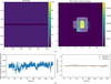
The radiation hardness of the JUNGFRAU allows us to record the direct beam and quantify its stability under typical 3D ED conditions. For each frame, the direct-beam spot is fitted with a rotated 2D super-Gaussian, and the beam intensity is defined as the integrated counts inside a 2σ ellipse around the fitted centroid [Fig. 3(a)]. The beam position remains stable within one pixel over a typical 3D ED data-collection time (∼3 min). The corresponding frame-to-frame fluctuations of the direct-beam intensity are limited to ∼2–3% relative standard deviation. Compared with the variation in effective crystal thickness during continuous rotation—often exceeding 100% over a tilt range of ∼60°—such intensity fluctuations are minor and can be sufficiently compensated for by scaling procedures in subsequent data-processing stages.
|
Figure 3
Static beam stability evaluated using the JUNGFRAU detector. (a) Definition of direct-beam properties using a 2D super-Gaussian fit (Ferjaoui et al., 2025 ). Beam intensity is quantified by integrating counts within the fitted elliptical region (right panel). (b) Temporal evolution of direct-beam intensity (left) and beam position (right) during continuous frame acquisition. To avoid pixel overload, data acquisition was performed at a reduced count rate corresponding to 1% of the standard configuration. |
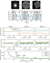
In the proposed workflow, the TEM magnification mode is switched frequently. Although this flexibility allows users to efficiently search for crystals and perform diffraction measurements, hysteresis effects in the electromagnetic lenses may induce unintended focus shifts, potentially requiring refocusing after each mode change. To evaluate focus reproducibility under such conditions, Fig. 4 presents an assessment using an aluminium standard grid. A series of image frames was recorded while repeatedly switching between DIFF, MAG and LowMAG modes. For frames acquired in DIFF mode, beam centering and focus quality were quantified using the direct-beam position and the intensities of major peaks in the aluminium Debye–Scherrer rings, respectively. Although the beam position exhibited shifts upon mode switching, the diffraction peak intensities remained largely consistent within the level of statistical fluctuation. This indicates that lens hysteresis is reproducible across the three magnification modes, and that a focusing operation to calibrate the focal plane is required only at the initial setup. Since the beam position is determined for each dataset in processing using the EPOC software suite (JFGui and PostprocessServer_JFED; see the following section), these positional shifts do not adversely affect subsequent data processing.
|
Figure 4
Beam focus reproducibility during magnification-mode switching. (a) (Top) Representative images acquired in DIFF, MAG and LowMAG modes, which are typically used for diffraction measurements, fine crystal alignment and crystal searching, respectively. (Bottom) Number of pixels detecting more than two electrons per frame in a continuous TEM image series, during which TEM modes were switched intermittently. As the illumination area depends on the TEM mode, the active mode can be identified on a per-frame basis, excluding intermediate transition frames. (b) Temporal evolution of the direct-beam position (top) and diffraction peak intensity (middle) for three frame subsets acquired in DIFF mode. The three major peaks in the azimuth integration profile (100, 200 and 220; bottom) are shown for comparison. These profiles mostly overlap, indicating stable focus reproduction despite multiple lens-current changes during mode switching. |
3.2. Crystallographic applications
3.2.1. Standard and applied use cases
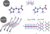
Fig. 5 presents the structures and the atomic charges determined through the proposed workflow. Histidine serves as a benchmark compound in 3D ED. Using the conventional neutral-atom model, residual negative features are observed between atoms in the difference electrostatic potential map, indicating valence electrons. Applying the iSFAC charged-atom model via ShelXFile_EDiSFAC, these residual features disappear [Figs. 5(a) and 5(b)], confirming the improved modeling of charge redistribution. Despite retaining spherical atomic scattering factors, iSFAC introduces one charge-transfer term per atom (Mahmoudi et al., 2025), yielding refined charges of +0.54 (5) for the amino group and −0.62 (5) for the carboxylate moiety. Because histidine is a chiral molecule and crystallized in a non-centrosymmetric space group (
P212121), the absolute configuration is chemically relevant. Using the DIALS output, dynamical refinement with JANA (Petříček et al., 2023) successfully established the L configuration, supported by the Z-score (Table 1) (Klar et al., 2023; Vypritskaia et al., 2025). This dynamical refinement step is not yet integrated into our standard workflow and currently requires manual processing. As in the previous study, data from multiple crystals were merged to reduce crystal-dependent variation; nevertheless, residual systematic effects from dynamical scattering cannot be quantified with the present procedure.
|
Figure 5
Structures resolved by the 3D ED workflow with JUNGFRAU. (a) Structure and electrostatic potential maps of L-histidine refined using conventional neutral-atom modeling. (b) Structure and maps after applying the iSFAC charged-atom model. The  maps are shown in blue (0.32 e− Å−1), and the  maps (−0.17 e− Å−1) are shown in red. In both cases, no continuous positive residual volume remains; in (b), negative residual volume is also absent. The inset in (b) shows the determined atomic charges. (c) Crystal structure of PTCDI-C8. The map (0.12 e− Å−1) is overlaid on the model at the center. (d) Determined atomic charges for PTCDI-C8. Half of the molecule is modeled on the basis of inversion symmetry. Partial sums of the alkyl and π-conjugated regions are indicated. The estimated standard deviations are displayed in parentheses. Insets in (a) and (c) show typical crystal images. 3D and 2D molecular pictures in (a–c) and (b, d) were created using ShelXle (Hübschle et al., 2011) and RDkit (Landrum, 2016), respectively. |
As a second sample, PTCDI-C8 is an organic semiconductor with a known triclinic structure determined previously by single-crystal X-ray diffraction (SXRD) at −143°C (Briseno et al., 2007). The workflow reproduced the same structure from nanowire crystals at room temperature, which are otherwise challenging for direct analysis. The determined atomic charges for the alkyl terminals and the π-conjugated core are +0.7 (2) and −0.7 (2), respectively, suggesting electron redistribution between these moieties [Figs. 5(c) and 5(d)]. This illustrates that the workflow can support both standard and advanced applications of 3D ED.
3.2.2. Data collection with high-speed rotation
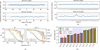
The JUNGFRAU detector supports data acquisition at 2 kHz, and in standard operation, images are summed over 20 frames for display and recording, corresponding to rotation slices of 0.025–0.10° at stage speeds of 0.5–2.0° s−1. This provides adequate sampling for typical organic crystals while extending dynamic range and reducing storage and graphic computation demands. To test the limits of the workflow, continuous-rotation datasets were collected at the JEM2100Plus stage's maximum nominal speed of 10° s−1. Fig. 6(a) compares nominal and readout values of rotation angles in single datasets collected at two different speeds. Approximately 10% deviation was observed at 10° s−1, in contrast to ∼1% at 2.0° s−1. This difference was reproducible across rotation, but the variance was not negligible [Fig. 6(b)]. In the post-processing pipeline (Section 2.2.4), the average of the readout values is used for each rotation, with outliers and systematic errors excluded.
|
Figure 6
Verification of high-speed continuous-rotation data collection. (a) Ratios of readout to nominal tilt angles during single rotation at nominal speeds of 2° s−1 (top) and 10° s−1 (bottom). The solid gray line represents the nominal value and the dashed line represents the mean value over the rotation. (b) Mean readout value for multiple independent rotations at 2° s−1 (top) and at 10° s−1 (bottom). The solid gray line represents the nominal value. (c) Statistics per resolution shell for L-histidine data collected at RT (left) and cryogenic (−110°C, right) conditions. The solid lines are CC1/2 on the right axes, and the dashed lines are for  on the left axes. (d) The determined bond lengths of L-histidine. The error bars indicate the estimated standard deviations. Background shading indicates bond types (carboxylic, aromatic and single). |
Figs. 6(c) and 6(d) show data statistics and refined bond lengths for L-histidine collected at 2.0 and 10° s−1 nominal rotation speed, under both room-temperature (RT) and cryogenic (−110°C) conditions. The beam illumination was adjusted to ∼1.3 e− Å−2 per crystal for either case. For RT data, high-speed acquisition produced slightly inferior statistics and one outlier bond length in the carboxylate group, probably due to crystal motion induced by higher instantaneous dose (Vlahakis et al., 2025; Vinothkumar & Henderson, 2016; Scheres, 2014). Cryogenic measurements suppressed this effect, yielding stable geometries even at 10° s−1. These results demonstrate that high-speed continuous rotation is feasible within the workflow, provided that the reduced dynamic range and increased per-second dose are considered.
A full ∼130° rotation can be acquired in ∼15 s, enabling rapid dataset collection which creates additional scope for obtaining more datasets and performing intermediate processing. Since the initial stage of the post-processing is sufficiently fast, indexing results are displayed before subsequent data collection starts. The time required for complete structure determination still depends on the performance of the downstream crystallographic programs.
3.2.3. Verification of beam-energy contribution
The JUNGFRAU detector and the workflow support data collection at various beam energies. In the previous study, we evaluated the spatial resolution of the JUNGFRAU over an electron energy range from 70 to 200 keV (Ferjaoui et al., 2025). There, higher spatial resolution was demonstrated at lower beam energies, owing to the reduced multiple scattering and lateral diffusion. The concept of exploiting lower-energy beams has also been proposed in imaging studies (Peet et al., 2019; Naydenova et al., 2019; McMullan et al., 2023).
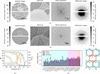
In Fig. 7, measurements with 100 and 200 kV beams are compared for perylene crystals, which are relatively radiation resistant due to the π-conjugated structure. Under illumination of the same electron count on the same crystal [Figs. 7(a) and 7(b)], the real-space image under the 100 kV beam exhibited higher contrast than that with the 200 kV beam, as highlighted in the power spectra. On the other hand, the diffraction image recorded at 200 kV exhibited substantially higher quality. This difference becomes more evident for collected 3D ED datasets. Despite comparable counts of electrons being exposed (∼6.5 e− Å−2 per crystal), the and CC1/2 statistics [Fig. 7(c)] were consistently superior for the 200 kV dataset, and the refined bond lengths agreed more closely with the SXRD reference structure (Näther et al., 1998). The two bridging C—C bonds between naphthalene units (C8—C18 and C10—C20) were distinguishable as single bonds at 200 kV, but not at 100 kV [Fig. 7(d)].
|
Figure 7
Real- and reciprocal-space resolution of perylene crystals measured with 100 and 200 kV electron beams. (a, b) Real-space (left) and diffraction (right) images of the same crystal acquired at 100 kV (a) and 200 kV (b). The two middle panels show a magnified view of a selected region in the real-space image and its corresponding power spectrum. The contrast scales are indicated by the bars on each side. The gray ring in the diffraction image indicates a resolution of 1 Å. (c) Dataset statistics per resolution shell. The solid lines are for CC1/2 on the right axes, and the dashed lines are for on the left axes. (d) The determined bond lengths. The error bars indicate the estimated standard deviation. For reference, the SXRD structure measured under room temperature from CCDC depositions is shown (Näther et al., 1998). Atomic labels correspond to the chemical formula in the right panel, and bonds are colored according to their environment. |
This behavior is primarily attributable to crystal thickness. The penetration depth of 100 kV electrons in graphite is 71 µm, in contrast to 233 µm at 200 kV (ICRU, 2014). Estimates that account for elastic and inelastic scattering contribution indicate that only crystals thinner than ∼65 nm (or ∼33 nm when tilted  60°) benefit from lower voltages (Peet et al., 2019). This requirement is stringent for diffraction measurement with the perylene crystals conducted here, and in practice, the higher-quality structure was obtained with the 200 kV beam, regardless of improved detector resolution. In general, the optimal accelerating voltage depends on both samples and microscopes. Factors such as the energy deposited by electrons in the sample, beam divergence and stability at different energies can also influence the quality of diffraction data.
4. Conclusions and outlook
In this work, we established an integrated hardware–software platform for 3D ED employing the JUNGFRAU 1M detector. The workflow combines the FPGA-based Jungfraujoch backend with the JFGui interface to coordinate the detector, microscope and processing modules in a unified environment. This integration enables fully synchronized data acquisition, metadata management and post-processing within a single, user-accessible framework. Application to L-histidine and PTCDI-C8 crystals demonstrated that structures can be resolved with charge-density evaluation using the iSFAC method, highlighting the system's capability for sub-atomic structural chemistry. Further assessments on broader classes of materials will extend the feasibility of this approach.
Beyond standard applications, the system performance was examined with respect to calibration accuracy, data-collection speed and beam-energy dependence. Continuous-rotation data collection at up to 10° s−1 was achieved without loss of data integrity, demonstrating the feasibility of high-throughput acquisition. The platform's compatibility with 100 and 200 keV beam energies revealed the practical trade-off between real-space contrast and reciprocal-space resolution, suggesting that lower-energy beams are expected to be adventageous for sufficiently thin specimens.
These developments represent important steps toward making 3D ED more practical and accessible through the use of the JUNGFRAU detector. By integrating high-speed data acquisition, adaptive calibration and live analysis into a cohesive workflow, the proposed platform shortens the experimental feedback cycle and reduces the practical effort required for routine 3D ED experiments. In particular, the integrated post-processing pipeline, together with immediate presentation of the processing results, allows users to evaluate data quality during acquisition and adapt the measurement strategy before collecting subsequent datasets, thereby improving the efficiency of data collection. This integrated workflow enables crystallographers to explore advanced methodology while also providing perspectives toward future instrument development.
This work in addition demonstrates a development model for emerging analytical techniques. Detector technologies have largely been advanced within large-scale facilities, particularly synchrotron and XFEL environments, where extensive resources are available. In contrast, the present platform was developed and validated within an in-house laboratory environment, illustrating how modern detector technologies can be translated into practical research tools outside major facilities. Such efforts are increasingly important for broadening access to advanced instrumentation and accelerating methodological dissemination.
Supporting information
Movie 1 Data collection using aluminum standard grid to create the calibration table. DOI: https://doi.org/10.1107/S1600576726009404/te5171sup1.mp4
Movie 2 Rotation data collection with live 3D spot plotting with JFGui. DOI: https://doi.org/10.1107/S1600576726009404/te5171sup2.mp4
Movie 3 Overlaid display of multiple diffraction datasets followed by their merging and phasing steps with JFGui. DOI: https://doi.org/10.1107/S1600576726009404/te5171sup3.mp4
Crystal structure: contains datablocks global, lhistidine-m110oC-2degs, lhistidine-m110oC-10degs, lhistidine-rt-2degs, lhistidine-rt-10degs, perylene-100kv, perylene-200kv, ptcdi-c8. DOI: https://doi.org/10.1107/S1600576726009404/te5171sup4.cif
Structure factors: contains datablock lhistidine-m110oC-2degs. DOI: https://doi.org/10.1107/S1600576726009404/te5171lhistidine-m110oC-2degssup5.hkl
Structure factors: contains datablock lhistidine-m110oC-10degs. DOI: https://doi.org/10.1107/S1600576726009404/te5171lhistidine-m110oC-10degssup6.hkl
Structure factors: contains datablock lhistidine-rt-2degs. DOI: https://doi.org/10.1107/S1600576726009404/te5171lhistidine-rt-2degssup7.hkl
Structure factors: contains datablock lhistidine-rt-10degs. DOI: https://doi.org/10.1107/S1600576726009404/te5171lhistidine-rt-10degssup8.hkl
Structure factors: contains datablock perylene-100kv. DOI: https://doi.org/10.1107/S1600576726009404/te5171perylene-100kvsup9.hkl
Structure factors: contains datablock perylene-200kv. DOI: https://doi.org/10.1107/S1600576726009404/te5171perylene-200kvsup10.hkl
Structure factors: contains datablock ptcdi-c8. DOI: https://doi.org/10.1107/S1600576726009404/te5171ptcdi-c8sup11.hkl
Supporting information file. DOI: https://doi.org/10.1107/S1600576726009404/te5171sup12.pdf
| C6H9N3O2 | F(000) = 122 |
| Mr = 155.16 | Dx = 1.448 Mg m−3 |
| Orthorhombic, P212121 | Electron radiation, λ = 0.02508 Å |
| a = 5.1576 (11) Å | Cell parameters from 4150 reflections |
| b = 7.307 (2) Å | θ = 1.2–0.1° |
| c = 18.888 (3) Å | µ = 0.00 mm−1 |
| V = 711.8 (3) Å3 | T = 163 K |
| Z = 4 | Block, colorless |
| Single axis tomography holder diffractometer | 1560 reflections with I > 2σ(I) |
| Radiation source: tansmission electron microscope, LaB6, JEOL JEM2100Plus | Rint = 0.210 |
| Detector resolution: 13.333 pixels mm-1 | θmax = 1.2°, θmin = 0.1° |
| profile fitting scans | h = −8→8 |
| 34103 measured reflections | k = −11→11 |
| 3189 independent reflections | l = −31→31 |
| Refinement on F2 | Primary atom site location: dual |
| Least-squares matrix: full | Hydrogen site location: inferred from neighbouring sites |
| R[F2 > 2σ(F2)] = 0.127 | H-atom parameters not defined |
| wR(F2) = 0.277 | w = 1/[σ2(Fo2) + (0.1P)2] where P = (Fo2 + 2Fc2)/3 |
| S = 1.21 | (Δ/σ)max < 0.001 |
| 3189 reflections | Δρmax = 0.15 e Å−3 |
| 147 parameters | Δρmin = −0.28 e Å−3 |
| 38 restraints | Absolute structure: All f" are zero, so absolute structure could not be determined |
Geometry. All esds (except the esd in the dihedral angle between two l.s. planes) are estimated using the full covariance matrix. The cell esds are taken into account individually in the estimation of esds in distances, angles and torsion angles; correlations between esds in cell parameters are only used when they are defined by crystal symmetry. An approximate (isotropic) treatment of cell esds is used for estimating esds involving l.s. planes. |
| x | y | z | Uiso*/Ueq | Occ. (<1) | |
| O1^a | 0.6741 (7) | 0.4964 (7) | 0.24086 (18) | 0.0383 (11) | 0.63 (3) |
| O2^a | 0.2729 (7) | 0.4988 (8) | 0.19829 (17) | 0.0420 (10) | 0.82 (3) |
| N1^a | 0.1276 (7) | 0.4999 (7) | 0.55351 (15) | 0.0367 (11) | 0.82 (3) |
| N2^a | −0.0324 (8) | 0.5592 (6) | 0.44712 (17) | 0.0361 (11) | 0.77 (3) |
| N3^a | 0.0867 (7) | 0.6827 (6) | 0.31104 (14) | 0.0304 (10) | 0.55 (3) |
| C1^a | 0.1960 (9) | 0.4596 (7) | 0.43859 (18) | 0.0368 (10) | 0.80 (3) |
| C2^a | −0.0629 (8) | 0.5816 (7) | 0.51676 (19) | 0.0408 (11) | 0.73 (3) |
| C3^a | 0.2966 (8) | 0.4233 (8) | 0.5055 (2) | 0.0394 (11) | 0.64 (3) |
| C4^a | 0.2925 (9) | 0.4094 (5) | 0.3670 (2) | 0.0417 (11) | 0.63 (4) |
| C5^a | 0.3343 (7) | 0.5798 (5) | 0.31959 (18) | 0.0362 (10) | 0.70 (3) |
| C6^a | 0.4364 (8) | 0.5222 (8) | 0.24631 (19) | 0.0374 (11) | 0.90 (3) |
| O1^b | 0.6741 (7) | 0.4964 (7) | 0.24086 (18) | 0.0383 (11) | 0.37 (3) |
| O2^b | 0.2729 (7) | 0.4988 (8) | 0.19829 (17) | 0.0420 (10) | 0.18 (3) |
| N1^b | 0.1276 (7) | 0.4999 (7) | 0.55351 (15) | 0.0367 (11) | 0.18 (3) |
| H2^b | 0.160 (3) | 0.513 (3) | 0.6071 (2) | 0.044* | 0.39 (2) |
| N2^b | −0.0324 (8) | 0.5592 (6) | 0.44712 (17) | 0.0361 (11) | 0.23 (3) |
| N3^b | 0.0867 (7) | 0.6827 (6) | 0.31104 (14) | 0.0304 (10) | 0.45 (3) |
| H3A^b | 0.1260 (11) | 0.8134 (8) | 0.2926 (4) | 0.046* | 0.32 (2) |
| H3B^b | −0.0069 (12) | 0.6911 (9) | 0.35946 (19) | 0.046* | 0.37 (2) |
| H3C^b | −0.0311 (8) | 0.6152 (12) | 0.2751 (3) | 0.046* | 0.32 (2) |
| C1^b | 0.1960 (9) | 0.4596 (7) | 0.43859 (18) | 0.0368 (10) | 0.20 (3) |
| C2^b | −0.0629 (8) | 0.5816 (7) | 0.51676 (19) | 0.0408 (11) | 0.27 (3) |
| H2A^b | −0.222 (4) | 0.655 (4) | 0.5412 (3) | 0.049* | 0.33 (2) |
| C3^b | 0.2966 (8) | 0.4233 (8) | 0.5055 (2) | 0.0394 (11) | 0.36 (3) |
| H3^b | 0.473 (3) | 0.350 (4) | 0.5179 (4) | 0.047* | 0.33 (2) |
| C4^b | 0.2925 (9) | 0.4094 (5) | 0.3670 (2) | 0.0417 (11) | 0.37 (4) |
| H4A^b | 0.1535 (19) | 0.3182 (9) | 0.3414 (3) | 0.050* | 0.31 (2) |
| H4B^b | 0.4757 (15) | 0.3357 (10) | 0.3721 (4) | 0.050* | 0.35 (2) |
| C5^b | 0.3343 (7) | 0.5798 (5) | 0.31959 (18) | 0.0362 (10) | 0.30 (3) |
| H5^b | 0.4782 (9) | 0.6693 (7) | 0.3448 (3) | 0.043* | 0.29 (2) |
| C6^b | 0.4364 (8) | 0.5222 (8) | 0.24631 (19) | 0.0374 (11) | 0.10 (3) |
| U11 | U22 | U33 | U12 | U13 | U23 | |
| O1^a | 0.0348 (19) | 0.042 (3) | 0.0379 (17) | 0.004 (2) | 0.0018 (12) | −0.0078 (16) |
| O2^a | 0.0421 (18) | 0.053 (3) | 0.0307 (15) | −0.004 (2) | 0.0012 (11) | −0.0044 (15) |
| N1^a | 0.044 (2) | 0.042 (3) | 0.0245 (15) | 0.002 (2) | −0.0003 (12) | −0.0006 (15) |
| N2^a | 0.040 (2) | 0.039 (3) | 0.0294 (17) | 0.0071 (19) | 0.0038 (13) | −0.0013 (15) |
| N3^a | 0.032 (2) | 0.030 (3) | 0.0289 (18) | 0.0007 (19) | −0.0026 (13) | 0.0007 (15) |
| C1^a | 0.046 (2) | 0.033 (3) | 0.0311 (17) | 0.005 (2) | 0.0030 (14) | 0.0021 (15) |
| C2^a | 0.046 (2) | 0.046 (3) | 0.0305 (18) | 0.004 (3) | 0.0015 (16) | −0.0029 (17) |
| C3^a | 0.043 (2) | 0.039 (3) | 0.0366 (19) | 0.009 (2) | 0.0005 (15) | 0.0017 (16) |
| C4^a | 0.050 (3) | 0.040 (3) | 0.035 (2) | 0.005 (2) | 0.0050 (17) | 0.0027 (18) |
| C5^a | 0.043 (2) | 0.035 (3) | 0.0308 (17) | 0.004 (2) | −0.0004 (14) | −0.0022 (15) |
| C6^a | 0.037 (2) | 0.044 (3) | 0.0314 (17) | −0.001 (2) | 0.0015 (14) | −0.0025 (16) |
| O1^b | 0.0348 (19) | 0.042 (3) | 0.0379 (17) | 0.004 (2) | 0.0018 (12) | −0.0078 (16) |
| O2^b | 0.0421 (18) | 0.053 (3) | 0.0307 (15) | −0.004 (2) | 0.0012 (11) | −0.0044 (15) |
| N1^b | 0.044 (2) | 0.042 (3) | 0.0245 (15) | 0.002 (2) | −0.0003 (12) | −0.0006 (15) |
| N2^b | 0.040 (2) | 0.039 (3) | 0.0294 (17) | 0.0071 (19) | 0.0038 (13) | −0.0013 (15) |
| N3^b | 0.032 (2) | 0.030 (3) | 0.0289 (18) | 0.0007 (19) | −0.0026 (13) | 0.0007 (15) |
| C1^b | 0.046 (2) | 0.033 (3) | 0.0311 (17) | 0.005 (2) | 0.0030 (14) | 0.0021 (15) |
| C2^b | 0.046 (2) | 0.046 (3) | 0.0305 (18) | 0.004 (3) | 0.0015 (16) | −0.0029 (17) |
| C3^b | 0.043 (2) | 0.039 (3) | 0.0366 (19) | 0.009 (2) | 0.0005 (15) | 0.0017 (16) |
| C4^b | 0.050 (3) | 0.040 (3) | 0.035 (2) | 0.005 (2) | 0.0050 (17) | 0.0027 (18) |
| C5^b | 0.043 (2) | 0.035 (3) | 0.0308 (17) | 0.004 (2) | −0.0004 (14) | −0.0022 (15) |
| C6^b | 0.037 (2) | 0.044 (3) | 0.0314 (17) | −0.001 (2) | 0.0015 (14) | −0.0025 (16) |
| O1a—C6a | 1.245 (6) | N1b—H2Ab | 2.143 (3) |
| O2a—C6a | 1.250 (5) | N1b—N2b | 2.215 (5) |
| N1a—C2a | 1.343 (4) | N1b—C1b | 2.219 (4) |
| N1a—C3a | 1.377 (4) | N2b—C2b | 1.335 (4) |
| N2a—C2a | 1.335 (4) | N2b—C1b | 1.394 (6) |
| N2a—C1a | 1.394 (6) | N2b—H3Bb | 1.920 (3) |
| N3a—C5a | 1.491 (3) | N2b—H2Ab | 2.145 (3) |
| C1a—C3a | 1.391 (4) | N2b—C3b | 2.254 (5) |
| C1a—C4a | 1.487 (5) | N2b—C4b | 2.510 (5) |
| C4a—C5a | 1.549 (5) | N2b—N3b | 2.793 (3) |
| C5a—C6a | 1.540 (5) | N3b—H3Ab | 1.0361 (13) |
| O1b—C6b | 1.245 (6) | N3b—H3Cb | 1.0362 (13) |
| O1b—H3Ab_$8i | 1.803 (6) | N3b—H3Bb | 1.0362 (13) |
| O1b—H3Cb_$6ii | 1.866 (6) | N3b—C5b | 1.491 (3) |
| O1b—O2b | 2.220 (5) | N3b—H5b | 2.120 (2) |
| O1b—C5b | 2.378 (5) | N3b—C6b | 2.474 (5) |
| O1b—N3b_$8i | 2.781 (6) | N3b—C4b | 2.497 (5) |
| O1b—N3b_$6ii | 2.853 (6) | C1b—C3b | 1.391 (4) |
| O2b—C6b | 1.250 (5) | C1b—C4b | 1.487 (5) |
| O2b—H2b_$5iii | 1.759 (5) | C2b—H2Ab | 1.0833 (13) |
| O2b—C5b | 2.388 (5) | C3b—H3b | 1.0829 (13) |
| O2b—N3b | 2.695 (4) | C4b—H4Ab | 1.0911 (14) |
| O2b—N1b_$5iii | 2.782 (4) | C4b—H4Bb | 1.0914 (14) |
| O2b—N3b_$7iv | 2.967 (6) | C4b—C5b | 1.549 (5) |
| N1b—H2b | 1.0299 (13) | C5b—H5b | 1.0981 (13) |
| N1b—C2b | 1.343 (4) | C5b—C6b | 1.540 (5) |
| N1b—C3b | 1.377 (4) | ||
| C2^a—N1^a—C3^a | 107.7 (2) | C5^b—N3^b—H5^b | 29.33 (8) |
| C2^a—N2^a—C1^a | 106.1 (3) | H3A^b—N3^b—C6^b | 97.4 (4) |
| C3^a—C1^a—N2^a | 108.0 (3) | H3C^b—N3^b—C6^b | 83.0 (2) |
| C3^a—C1^a—C4^a | 130.8 (3) | H3B^b—N3^b—C6^b | 143.5 (3) |
| N2^a—C1^a—C4^a | 121.1 (4) | C5^b—N3^b—C6^b | 35.91 (16) |
| N2^a—C2^a—N1^a | 111.6 (3) | H5^b—N3^b—C6^b | 55.44 (12) |
| N1^a—C3^a—C1^a | 106.5 (2) | H3A^b—N3^b—C4^b | 142.8 (2) |
| C1^a—C4^a—C5^a | 111.9 (3) | H3C^b—N3^b—C4^b | 98.4 (4) |
| N3^a—C5^a—C6^a | 109.5 (3) | H3B^b—N3^b—C4^b | 82.6 (3) |
| N3^a—C5^a—C4^a | 110.4 (3) | C5^b—N3^b—C4^b | 35.55 (16) |
| C6^a—C5^a—C4^a | 110.3 (3) | H5^b—N3^b—C4^b | 55.30 (12) |
| O1^a—C6^a—O2^a | 125.7 (4) | C6^b—N3^b—C4^b | 61.32 (16) |
| O1^a—C6^a—C5^a | 116.9 (3) | H3A^b—N3^b—O2^b | 97.2 (5) |
| O2^a—C6^a—C5^a | 117.3 (4) | H3C^b—N3^b—O2^b | 56.9 (2) |
| C6^b—O1^b—H3C^b_$6^ii^ | 134.7 (4) | H3B^b—N3^b—O2^b | 153.2 (5) |
| H3A^b^i^—O1^b—H3C^b_$6^ii^ | 90.1 (3) | C5^b—N3^b—O2^b | 61.89 (16) |
| C6^b—O1^b—O2^b | 27.2 (2) | H5^b—N3^b—O2^b | 82.86 (16) |
| H3A^b^i^—O1^b—O2^b | 114.3 (3) | C6^b—N3^b—O2^b | 27.57 (12) |
| H3C^b^ii^—O1^b—O2^b | 151.8 (4) | C4^b—N3^b—O2^b | 77.52 (16) |
| C6^b—O1^b—C5^b | 35.3 (2) | H3A^b—N3^b—N2^b | 130.5 (4) |
| H3A^b^i^—O1^b—C5^b | 146.2 (4) | H3C^b—N3^b—N2^b | 108.7 (4) |
| H3C^b^ii^—O1^b—C5^b | 105.3 (2) | H3B^b—N3^b—N2^b | 26.4 (3) |
| O2^b—O1^b—C5^b | 62.45 (15) | C5^b—N3^b—N2^b | 85.74 (18) |
| C6^b—O2^b—O1^b | 27.1 (2) | H5^b—N3^b—N2^b | 85.3 (2) |
| H2^b^iii^—O2^b—O1^b | 99.9 (5) | C6^b—N3^b—N2^b | 117.51 (18) |
| C6^b—O2^b—C5^b | 34.9 (2) | C4^b—N3^b—N2^b | 56.32 (14) |
| H2^b^iii^—O2^b—C5^b | 157.8 (9) | O2^b—N3^b—N2^b | 130.1 (2) |
| O1^b—O2^b—C5^b | 62.02 (15) | O1^b^v^—N3^b—N2^b | 133.50 (19) |
| C6^b—O2^b—N3^b | 66.3 (3) | N3^b—H3B^b—N2^b | 139.8 (4) |
| H2^b^iii^—O2^b—N3^b | 150.2 (6) | C3^b—C1^b—N2^b | 108.0 (3) |
| O1^b—O2^b—N3^b | 92.86 (18) | C3^b—C1^b—C4^b | 130.8 (3) |
| C5^b—O2^b—N3^b | 33.42 (8) | N2^b—C1^b—C4^b | 121.1 (4) |
| H2^b—N1^b—C2^b | 125.8 (4) | C3^b—C1^b—N1^b | 36.52 (18) |
| H2^b—N1^b—C3^b | 125.6 (4) | N2^b—C1^b—N1^b | 71.5 (2) |
| C2^b—N1^b—C3^b | 107.7 (2) | C4^b—C1^b—N1^b | 167.4 (3) |
| H2^b—N1^b—H2A^b | 101.2 (5) | H2A^b—C2^b—N2^b | 124.7 (4) |
| C2^b—N1^b—H2A^b | 24.88 (15) | H2A^b—C2^b—N1^b | 123.7 (4) |
| C3^b—N1^b—H2A^b | 132.5 (2) | N2^b—C2^b—N1^b | 111.6 (3) |
| H2^b—N1^b—N2^b | 159.0 (7) | C2^b—H2A^b—N1^b | 31.4 (3) |
| C2^b—N1^b—N2^b | 34.07 (15) | C2^b—H2A^b—N2^b | 30.8 (3) |
| C3^b—N1^b—N2^b | 73.6 (2) | N1^b—H2A^b—N2^b | 62.21 (15) |
| H2A^b—N1^b—N2^b | 58.96 (11) | H3^b—C3^b—N1^b | 126.2 (4) |
| H2^b—N1^b—C1^b | 161.3 (7) | H3^b—C3^b—C1^b | 127.2 (5) |
| C2^b—N1^b—C1^b | 70.7 (2) | N1^b—C3^b—C1^b | 106.5 (2) |
| C3^b—N1^b—C1^b | 36.93 (15) | H3^b—C3^b—N2^b | 163.2 (5) |
| H2A^b—N1^b—C1^b | 95.6 (2) | N1^b—C3^b—N2^b | 70.52 (19) |
| N2^b—N1^b—C1^b | 36.66 (15) | C1^b—C3^b—N2^b | 36.03 (18) |
| C2^b—N2^b—C1^b | 106.1 (3) | H4A^b—C4^b—H4B^b | 107.8 (2) |
| C2^b—N2^b—H3B^b | 142.8 (4) | H4A^b—C4^b—C1^b | 109.5 (4) |
| C1^b—N2^b—H3B^b | 96.0 (3) | H4B^b—C4^b—C1^b | 109.4 (4) |
| C2^b—N2^b—H2A^b | 24.52 (16) | H4A^b—C4^b—C5^b | 109.1 (4) |
| C1^b—N2^b—H2A^b | 130.6 (3) | H4B^b—C4^b—C5^b | 109.1 (4) |
| H3B^b—N2^b—H2A^b | 125.5 (6) | C1^b—C4^b—C5^b | 111.9 (3) |
| C2^b—N2^b—N1^b | 34.32 (19) | H4A^b—C4^b—N3^b | 91.3 (3) |
| C1^b—N2^b—N1^b | 71.8 (2) | H4B^b—C4^b—N3^b | 143.1 (4) |
| H3B^b—N2^b—N1^b | 148.7 (4) | C1^b—C4^b—N3^b | 92.6 (2) |
| H2A^b—N2^b—N1^b | 58.84 (11) | C5^b—C4^b—N3^b | 34.03 (15) |
| C2^b—N2^b—C3^b | 70.2 (2) | H4A^b—C4^b—N2^b | 95.4 (4) |
| C1^b—N2^b—C3^b | 35.9 (2) | H4B^b—C4^b—N2^b | 137.8 (4) |
| H3B^b—N2^b—C3^b | 126.2 (3) | C1^b—C4^b—N2^b | 28.4 (2) |
| H2A^b—N2^b—C3^b | 94.7 (2) | C5^b—C4^b—N2^b | 95.2 (2) |
| N1^b—N2^b—C3^b | 35.89 (13) | N3^b—C4^b—N2^b | 67.81 (13) |
| C2^b—N2^b—C4^b | 136.6 (3) | H5^b—C5^b—N3^b | 109.0 (2) |
| C1^b—N2^b—C4^b | 30.5 (2) | H5^b—C5^b—C6^b | 108.8 (4) |
| H3B^b—N2^b—C4^b | 69.7 (2) | N3^b—C5^b—C6^b | 109.5 (3) |
| H2A^b—N2^b—C4^b | 161.1 (3) | H5^b—C5^b—C4^b | 108.8 (3) |
| N1^b—N2^b—C4^b | 102.3 (2) | N3^b—C5^b—C4^b | 110.4 (3) |
| C3^b—N2^b—C4^b | 66.41 (18) | C6^b—C5^b—C4^b | 110.3 (3) |
| C2^b—N2^b—N3^b | 153.3 (4) | H5^b—C5^b—O1^b | 85.8 (3) |
| C1^b—N2^b—N3^b | 82.9 (2) | N3^b—C5^b—O1^b | 133.9 (2) |
| H3B^b—N2^b—N3^b | 13.87 (13) | C6^b—C5^b—O1^b | 27.82 (19) |
| H2A^b—N2^b—N3^b | 139.2 (7) | C4^b—C5^b—O1^b | 104.9 (2) |
| N1^b—N2^b—N3^b | 144.7 (2) | H5^b—C5^b—O2^b | 130.9 (4) |
| C3^b—N2^b—N3^b | 115.26 (19) | N3^b—C5^b—O2^b | 84.69 (17) |
| C4^b—N2^b—N3^b | 55.88 (14) | C6^b—C5^b—O2^b | 27.72 (19) |
| H3A^b—N3^b—H3C^b | 109.5 (2) | C4^b—C5^b—O2^b | 109.7 (2) |
| H3A^b—N3^b—H3B^b | 109.5 (2) | O1^b—C5^b—O2^b | 55.53 (15) |
| H3C^b—N3^b—H3B^b | 109.4 (2) | C5^b—H5^b—N3^b | 41.69 (16) |
| H3A^b—N3^b—C5^b | 109.5 (2) | O1^b—C6^b—O2^b | 125.7 (4) |
| H3C^b—N3^b—C5^b | 109.5 (2) | O1^b—C6^b—C5^b | 116.9 (3) |
| H3B^b—N3^b—C5^b | 109.5 (2) | O2^b—C6^b—C5^b | 117.3 (4) |
| H3A^b—N3^b—H5^b | 87.58 (16) | O1^b—C6^b—N3^b | 146.2 (3) |
| H3C^b—N3^b—H5^b | 137.2 (2) | O2^b—C6^b—N3^b | 86.1 (3) |
| H3B^b—N3^b—H5^b | 100.4 (4) | C5^b—C6^b—N3^b | 34.61 (15) |
| C2a—N2a—C1a—C3a | 0.5 (6) | N1b—C1b—C4b—N2b | 178 (2) |
| C2a—N2a—C1a—C4a | −179.7 (4) | H3Ab—N3b—C5b—H5b | 43.8 (6) |
| C1a—N2a—C2a—N1a | −1.3 (6) | H3Cb—N3b—C5b—H5b | 163.8 (5) |
| C3a—N1a—C2a—N2a | 1.6 (7) | H3Bb—N3b—C5b—H5b | −76.2 (6) |
| C2a—N1a—C3a—C1a | −1.2 (6) | C6b—N3b—C5b—H5b | 118.9 (4) |
| N2a—C1a—C3a—N1a | 0.4 (6) | C4b—N3b—C5b—H5b | −119.4 (5) |
| C4a—C1a—C3a—N1a | −179.3 (5) | O2b—N3b—C5b—H5b | 131.5 (4) |
| C3a—C1a—C4a—C5a | −123.0 (6) | O1bv—N3b—C5b—H5b | 45.5 (4) |
| N2a—C1a—C4a—C5a | 57.3 (6) | N2b—N3b—C5b—H5b | −87.9 (4) |
| C1a—C4a—C5a—N3a | −59.4 (4) | O1bvi—N3b—C5b—H5b | 177.2 (4) |
| C1a—C4a—C5a—C6a | 179.5 (4) | O2bvii—N3b—C5b—H5b | 18.3 (8) |
| N3a—C5a—C6a—O1a | 154.8 (5) | H3Ab—N3b—C5b—C6b | −75.1 (6) |
| C4a—C5a—C6a—O1a | −83.5 (5) | H3Cb—N3b—C5b—C6b | 44.9 (5) |
| N3a—C5a—C6a—O2a | −27.9 (6) | H3Bb—N3b—C5b—C6b | 164.9 (5) |
| C4a—C5a—C6a—O2a | 93.8 (6) | H5b—N3b—C5b—C6b | −118.9 (4) |
| H3Cb—N3b—H3Ab—O1bv | −113.7 (18) | C4b—N3b—C5b—C6b | 121.7 (3) |
| H3Bb—N3b—H3Ab—O1bv | 126.4 (19) | O2b—N3b—C5b—C6b | 12.6 (3) |
| C5b—N3b—H3Ab—O1bv | 6.3 (19) | O1bv—N3b—C5b—C6b | −73.4 (3) |
| H5b—N3b—H3Ab—O1bv | 26.2 (17) | N2b—N3b—C5b—C6b | 153.2 (3) |
| C6b—N3b—H3Ab—O1bv | −28.5 (18) | O1bvi—N3b—C5b—C6b | 58.3 (3) |
| C4b—N3b—H3Ab—O1bv | 22 (2) | O2bvii—N3b—C5b—C6b | −100.6 (5) |
| O2b—N3b—H3Ab—O1bv | −56.3 (18) | H3Ab—N3b—C5b—C4b | 163.2 (5) |
| N2b—N3b—H3Ab—O1bv | 107.8 (17) | H3Cb—N3b—C5b—C4b | −76.8 (5) |
| O1bvi—N3b—H3Ab—O1bv | −127.7 (16) | H3Bb—N3b—C5b—C4b | 43.2 (5) |
| O2bvii—N3b—H3Ab—O1bv | 175 (2) | H5b—N3b—C5b—C4b | 119.4 (5) |
| H3Ab—N3b—H3Bb—N2b | −147.0 (9) | C6b—N3b—C5b—C4b | −121.7 (3) |
| H3Cb—N3b—H3Bb—N2b | 93.0 (11) | O2b—N3b—C5b—C4b | −109.0 (3) |
| C5b—N3b—H3Bb—N2b | −27.0 (10) | O1bv—N3b—C5b—C4b | 164.9 (2) |
| H5b—N3b—H3Bb—N2b | −55.9 (10) | N2b—N3b—C5b—C4b | 31.5 (2) |
| C6b—N3b—H3Bb—N2b | −12.1 (15) | O1bvi—N3b—C5b—C4b | −63.3 (3) |
| C4b—N3b—H3Bb—N2b | −3.3 (8) | O2bvii—N3b—C5b—C4b | 137.8 (5) |
| O2b—N3b—H3Bb—N2b | 38.9 (14) | H3Ab—N3b—C5b—O1b | −59.1 (6) |
| O1bv—N3b—H3Bb—N2b | −133.1 (8) | H3Cb—N3b—C5b—O1b | 60.9 (5) |
| O1bvi—N3b—H3Bb—N2b | 93.6 (8) | H3Bb—N3b—C5b—O1b | −179.1 (5) |
| O2bvii—N3b—H3Bb—N2b | 174.7 (10) | H5b—N3b—C5b—O1b | −102.9 (5) |
| H3Ab—N3b—H3Cb—O1bvi | −117.3 (15) | C6b—N3b—C5b—O1b | 16.0 (3) |
| H3Bb—N3b—H3Cb—O1bvi | 2.7 (16) | C4b—N3b—C5b—O1b | 137.7 (4) |
| C5b—N3b—H3Cb—O1bvi | 122.7 (15) | O2b—N3b—C5b—O1b | 28.7 (3) |
| H5b—N3b—H3Cb—O1bvi | 134.3 (13) | O1bv—N3b—C5b—O1b | −57.4 (3) |
| C6b—N3b—H3Cb—O1bvi | 147.3 (17) | N2b—N3b—C5b—O1b | 169.2 (3) |
| C4b—N3b—H3Cb—O1bvi | 87.8 (16) | O1bvi—N3b—C5b—O1b | 74.3 (3) |
| O2b—N3b—H3Cb—O1bvi | 156.9 (19) | O2bvii—N3b—C5b—O1b | −84.6 (6) |
| O1bv—N3b—H3Cb—O1bvi | −132.8 (16) | H3Ab—N3b—C5b—O2b | −87.7 (5) |
| N2b—N3b—H3Cb—O1bvi | 30.6 (17) | H3Cb—N3b—C5b—O2b | 32.3 (5) |
| O2bvii—N3b—H3Cb—O1bvi | −69.0 (16) | H3Bb—N3b—C5b—O2b | 152.2 (5) |
| C2b—N2b—C1b—C3b | 0.5 (6) | H5b—N3b—C5b—O2b | −131.5 (4) |
| H3Bb—N2b—C1b—C3b | 150.2 (5) | C6b—N3b—C5b—O2b | −12.6 (3) |
| H2Ab—N2b—C1b—C3b | 0.9 (14) | C4b—N3b—C5b—O2b | 109.0 (3) |
| N1b—N2b—C1b—C3b | −0.3 (4) | O1bv—N3b—C5b—O2b | −86.06 (18) |
| C4b—N2b—C1b—C3b | −179.8 (7) | N2b—N3b—C5b—O2b | 140.6 (2) |
| N3b—N2b—C1b—C3b | 154.8 (4) | O1bvi—N3b—C5b—O2b | 45.7 (2) |
| C2b—N2b—C1b—C4b | −179.7 (4) | O2bvii—N3b—C5b—O2b | −113.2 (5) |
| H3Bb—N2b—C1b—C4b | −30.0 (5) | H4Ab—C4b—C5b—H5b | −178.5 (6) |
| H2Ab—N2b—C1b—C4b | −179.4 (13) | H4Bb—C4b—C5b—H5b | −61.0 (6) |
| N1b—N2b—C1b—C4b | 179.5 (5) | C1b—C4b—C5b—H5b | 60.2 (5) |
| C3b—N2b—C1b—C4b | 179.8 (7) | N3b—C4b—C5b—H5b | 119.6 (4) |
| N3b—N2b—C1b—C4b | −25.5 (4) | N2b—C4b—C5b—H5b | 83.9 (4) |
| C2b—N2b—C1b—N1b | 0.8 (4) | H4Ab—C4b—C5b—N3b | 61.9 (5) |
| H3Bb—N2b—C1b—N1b | 150.5 (4) | H4Bb—C4b—C5b—N3b | 179.5 (5) |
| H2Ab—N2b—C1b—N1b | 1.1 (13) | C1b—C4b—C5b—N3b | −59.4 (4) |
| C3b—N2b—C1b—N1b | 0.3 (4) | N2b—C4b—C5b—N3b | −35.6 (3) |
| C4b—N2b—C1b—N1b | −179.5 (5) | H4Ab—C4b—C5b—C6b | −59.2 (5) |
| N3b—N2b—C1b—N1b | 155.0 (2) | H4Bb—C4b—C5b—C6b | 58.3 (5) |
| C1b—N2b—C2b—H2Ab | 179 (2) | C1b—C4b—C5b—C6b | 179.5 (4) |
| H3Bb—N2b—C2b—H2Ab | 55 (2) | N3b—C4b—C5b—C6b | −121.2 (3) |
| N1b—N2b—C2b—H2Ab | −179 (2) | N2b—C4b—C5b—C6b | −156.8 (3) |
| C3b—N2b—C2b—H2Ab | 180 (2) | H4Ab—C4b—C5b—O1b | −87.9 (4) |
| C4b—N2b—C2b—H2Ab | 179 (2) | H4Bb—C4b—C5b—O1b | 29.6 (5) |
| N3b—N2b—C2b—H2Ab | 73 (2) | C1b—C4b—C5b—O1b | 150.8 (3) |
| C1b—N2b—C2b—N1b | −1.3 (6) | N3b—C4b—C5b—O1b | −149.8 (3) |
| H3Bb—N2b—C2b—N1b | −125.3 (6) | N2b—C4b—C5b—O1b | 174.51 (19) |
| H2Ab—N2b—C2b—N1b | 179 (2) | H4Ab—C4b—C5b—O2b | −29.7 (5) |
| C3b—N2b—C2b—N1b | −1.0 (4) | H4Bb—C4b—C5b—O2b | 87.9 (4) |
| C4b—N2b—C2b—N1b | −1.5 (8) | C1b—C4b—C5b—O2b | −151.0 (3) |
| N3b—N2b—C2b—N1b | −108.0 (7) | N3b—C4b—C5b—O2b | −91.6 (2) |
| H2b—N1b—C2b—H2Ab | −10 (3) | N2b—C4b—C5b—O2b | −127.3 (2) |
| C3b—N1b—C2b—H2Ab | −179 (2) | C6b—C5b—H5b—N3b | 119.3 (4) |
| N2b—N1b—C2b—H2Ab | 179 (2) | C4b—C5b—H5b—N3b | −120.5 (4) |
| C1b—N1b—C2b—H2Ab | −180 (2) | O1b—C5b—H5b—N3b | 135.2 (3) |
| O2bviii—N1b—C2b—H2Ab | −5 (2) | O2b—C5b—H5b—N3b | 99.7 (4) |
| H2b—N1b—C2b—N2b | 171.1 (19) | H3Abi—O1b—C6b—O2b | −48.5 (10) |
| C3b—N1b—C2b—N2b | 1.6 (7) | H3Cbii—O1b—C6b—O2b | 141.9 (6) |
| H2Ab—N1b—C2b—N2b | −179 (2) | C5b—O1b—C6b—O2b | −177.1 (10) |
| C1b—N1b—C2b—N2b | 0.8 (4) | N3bi—O1b—C6b—O2b | −50.8 (8) |
| O2bviii—N1b—C2b—N2b | 175.3 (4) | N3bii—O1b—C6b—O2b | 148.6 (5) |
| N2b—C2b—H2Ab—N1b | 179 (3) | H3Abi—O1b—C6b—C5b | 128.6 (6) |
| N1b—C2b—H2Ab—N2b | −179 (3) | H3Cbii—O1b—C6b—C5b | −41.0 (9) |
| H2b—N1b—C3b—H3b | 9 (3) | O2b—O1b—C6b—C5b | 177.1 (10) |
| C2b—N1b—C3b—H3b | 179 (2) | N3bi—O1b—C6b—C5b | 126.3 (3) |
| H2Ab—N1b—C3b—H3b | 178 (3) | N3bii—O1b—C6b—C5b | −34.3 (7) |
| N2b—N1b—C3b—H3b | 180 (2) | H3Abi—O1b—C6b—N3b | 154.4 (6) |
| C1b—N1b—C3b—H3b | 180 (2) | H3Cbii—O1b—C6b—N3b | −15.2 (11) |
| O2bviii—N1b—C3b—H3b | 4 (2) | O2b—O1b—C6b—N3b | −157.1 (12) |
| H2b—N1b—C3b—C1b | −170.7 (19) | C5b—O1b—C6b—N3b | 25.8 (4) |
| C2b—N1b—C3b—C1b | −1.2 (6) | N3bi—O1b—C6b—N3b | 152.1 (5) |
| H2Ab—N1b—C3b—C1b | −1.7 (14) | N3bii—O1b—C6b—N3b | −8.5 (10) |
| N2b—N1b—C3b—C1b | −0.3 (4) | H2biii—O2b—C6b—O1b | −19.0 (13) |
| O2bviii—N1b—C3b—C1b | −175.5 (4) | C5b—O2b—C6b—O1b | 177.1 (10) |
| H2b—N1b—C3b—N2b | −170.5 (19) | N3b—O2b—C6b—O1b | −167.5 (7) |
| C2b—N1b—C3b—N2b | −0.9 (4) | N1biii—O2b—C6b—O1b | −22.8 (9) |
| H2Ab—N1b—C3b—N2b | −1.5 (13) | N3biv—O2b—C6b—O1b | 103.8 (6) |
| C1b—N1b—C3b—N2b | 0.3 (4) | H2biii—O2b—C6b—C5b | 163.9 (10) |
| O2bviii—N1b—C3b—N2b | −175.2 (4) | O1b—O2b—C6b—C5b | −177.1 (10) |
| N2b—C1b—C3b—H3b | −179 (2) | N3b—O2b—C6b—C5b | 15.5 (3) |
| C4b—C1b—C3b—H3b | 1 (2) | N1biii—O2b—C6b—C5b | 160.1 (3) |
| N1b—C1b—C3b—H3b | −180 (2) | N3biv—O2b—C6b—C5b | −73.3 (6) |
| N2b—C1b—C3b—N1b | 0.4 (6) | H2biii—O2b—C6b—N3b | 148.5 (10) |
| C4b—C1b—C3b—N1b | −179.3 (5) | O1b—O2b—C6b—N3b | 167.5 (7) |
| C4b—C1b—C3b—N2b | −179.7 (8) | C5b—O2b—C6b—N3b | −15.5 (3) |
| N1b—C1b—C3b—N2b | −0.4 (6) | N1biii—O2b—C6b—N3b | 144.7 (4) |
| C3b—C1b—C4b—H4Ab | 116.0 (6) | N3biv—O2b—C6b—N3b | −88.7 (3) |
| N2b—C1b—C4b—H4Ab | −63.7 (7) | H5b—C5b—C6b—O1b | 35.8 (6) |
| N1b—C1b—C4b—H4Ab | 114.1 (16) | N3b—C5b—C6b—O1b | 154.8 (5) |
| C3b—C1b—C4b—H4Bb | −2.0 (7) | C4b—C5b—C6b—O1b | −83.5 (5) |
| N2b—C1b—C4b—H4Bb | 178.3 (6) | O2b—C5b—C6b—O1b | −177.3 (9) |
| N1b—C1b—C4b—H4Bb | −3.9 (17) | H5b—C5b—C6b—O2b | −146.9 (5) |
| C3b—C1b—C4b—C5b | −123.0 (6) | N3b—C5b—C6b—O2b | −27.9 (6) |
| N2b—C1b—C4b—C5b | 57.3 (6) | C4b—C5b—C6b—O2b | 93.8 (6) |
| N1b—C1b—C4b—C5b | −124.8 (16) | O1b—C5b—C6b—O2b | 177.3 (9) |
| C3b—C1b—C4b—N3b | −151.8 (6) | H5b—C5b—C6b—N3b | −119.0 (3) |
| N2b—C1b—C4b—N3b | 28.5 (5) | C4b—C5b—C6b—N3b | 121.7 (3) |
| N1b—C1b—C4b—N3b | −153.7 (17) | O1b—C5b—C6b—N3b | −154.8 (5) |
| C3b—C1b—C4b—N2b | 179.7 (9) | O2b—C5b—C6b—N3b | 27.9 (6) |
| Symmetry codes: (i) −x+1, y−1/2, −z+1/2; (ii) x+1, y, z; (iii) −x+1/2, −y+1, z−1/2; (iv) −x, y−1/2, −z+1/2; (v) −x+1, y+1/2, −z+1/2; (vi) x−1, y, z; (vii) −x, y+1/2, −z+1/2; (viii) −x+1/2, −y+1, z+1/2. |
| C6H9N3O2 | F(000) = 122 |
| Mr = 155.16 | Dx = 1.384 Mg m−3 |
| Orthorhombic, P212121 | Cell parameters from 59288 reflections |
| a = 5.2601 (13) Å | θ = 0.1–1.2° |
| b = 7.4275 (18) Å | µ = 0.00 mm−1 |
| c = 19.062 (4) Å | T = 163 K |
| V = 744.7 (3) Å3 | Block, colorless |
| Z = 4 |
| Single axis tomography holder diffractometer | 1951 reflections with I > 2σ(I) |
| Radiation source: tansmission electron microscope, LaB6, JEOL JEM2100Plus | Rint = 0.481 |
| Detector resolution: 13.333 pixels mm-1 | θmax = 1.2°, θmin = 0.1° |
| profile fitting scans | h = −8→8 |
| 59288 measured reflections | k = −12→12 |
| 3451 independent reflections | l = −31→31 |
| Refinement on F2 | Primary atom site location: dual |
| Least-squares matrix: full | Hydrogen site location: inferred from neighbouring sites |
| R[F2 > 2σ(F2)] = 0.136 | H-atom parameters not defined |
| wR(F2) = 0.319 | w = 1/[σ2(Fo2) + (0.1P)2] where P = (Fo2 + 2Fc2)/3 |
| S = 1.35 | (Δ/σ)max < 0.001 |
| 3451 reflections | Δρmax = 0.17 e Å−3 |
| 147 parameters | Δρmin = −0.25 e Å−3 |
| 38 restraints | Absolute structure: All f" are zero, so absolute structure could not be determined |
Geometry. All esds (except the esd in the dihedral angle between two l.s. planes) are estimated using the full covariance matrix. The cell esds are taken into account individually in the estimation of esds in distances, angles and torsion angles; correlations between esds in cell parameters are only used when they are defined by crystal symmetry. An approximate (isotropic) treatment of cell esds is used for estimating esds involving l.s. planes. |
| x | y | z | Uiso*/Ueq | Occ. (<1) | |
| O2 | −0.2743 (7) | −0.5043 (9) | −0.1985 (2) | 0.0580 (11) | 0.75 (3) |
| O1 | −0.6739 (7) | −0.5074 (6) | −0.2413 (2) | 0.0506 (10) | 0.60 (3) |
| N1 | −0.1269 (7) | −0.5004 (6) | −0.55396 (18) | 0.0498 (11) | 0.80 (3) |
| N2 | 0.0326 (8) | −0.4409 (6) | −0.4471 (2) | 0.0464 (11) | 0.70 (2) |
| N3 | −0.0876 (7) | −0.3202 (5) | −0.31056 (16) | 0.0439 (10) | 0.60 (3) |
| C1 | −0.1951 (9) | −0.5394 (7) | −0.4392 (2) | 0.0527 (9) | 0.79 (3) |
| C3 | −0.2962 (9) | −0.5759 (8) | −0.5060 (2) | 0.0572 (11) | 0.61 (4) |
| C2 | 0.0600 (9) | −0.4208 (8) | −0.5168 (2) | 0.0562 (11) | 0.67 (4) |
| C4 | −0.2906 (10) | −0.5912 (5) | −0.3668 (3) | 0.0551 (10) | 0.70 (4) |
| C5 | −0.3328 (6) | −0.4217 (5) | −0.3198 (2) | 0.0482 (8) | 0.65 (4) |
| C6 | −0.4369 (9) | −0.4817 (7) | −0.2463 (2) | 0.0522 (9) | 0.94 (3) |
| O2 | −0.2743 (7) | −0.5043 (9) | −0.1985 (2) | 0.0580 (11) | 0.25 (3) |
| O1 | −0.6739 (7) | −0.5074 (6) | −0.2413 (2) | 0.0506 (10) | 0.40 (3) |
| N1 | −0.1269 (7) | −0.5004 (6) | −0.55396 (18) | 0.0498 (11) | 0.20 (3) |
| H1 | −0.158 (3) | −0.487 (4) | −0.6070 (3) | 0.060* | 0.35 (2) |
| N2 | 0.0326 (8) | −0.4409 (6) | −0.4471 (2) | 0.0464 (11) | 0.30 (2) |
| N3 | −0.0876 (7) | −0.3202 (5) | −0.31056 (16) | 0.0439 (10) | 0.40 (3) |
| H3A | 0.0026 (12) | −0.3077 (9) | −0.35864 (19) | 0.066* | 0.42 (2) |
| H3B | 0.0292 (8) | −0.3896 (12) | −0.2761 (3) | 0.066* | 0.25 (2) |
| H3C | −0.1257 (11) | −0.1934 (8) | −0.2905 (4) | 0.066* | 0.33 (3) |
| C1 | −0.1951 (9) | −0.5394 (7) | −0.4392 (2) | 0.0527 (9) | 0.21 (3) |
| C3 | −0.2962 (9) | −0.5759 (8) | −0.5060 (2) | 0.0572 (11) | 0.39 (4) |
| H3 | −0.476 (3) | −0.640 (4) | −0.5183 (4) | 0.069* | 0.39 (3) |
| C2 | 0.0600 (9) | −0.4208 (8) | −0.5168 (2) | 0.0562 (11) | 0.33 (4) |
| H2 | 0.220 (4) | −0.353 (4) | −0.5410 (3) | 0.067* | 0.32 (3) |
| C4 | −0.2906 (10) | −0.5912 (5) | −0.3668 (3) | 0.0551 (10) | 0.30 (4) |
| H4A | −0.153 (2) | −0.6799 (9) | −0.3415 (3) | 0.066* | 0.26 (3) |
| H4B | −0.4695 (16) | −0.6644 (11) | −0.3717 (4) | 0.066* | 0.33 (3) |
| C5 | −0.3328 (6) | −0.4217 (5) | −0.3198 (2) | 0.0482 (8) | 0.35 (4) |
| H5 | −0.4728 (9) | −0.3335 (7) | −0.3452 (3) | 0.058* | 0.30 (3) |
| C6 | −0.4369 (9) | −0.4817 (7) | −0.2463 (2) | 0.0522 (9) | 0.06 (3) |
| U11 | U22 | U33 | U12 | U13 | U23 | |
| O2 | 0.0496 (17) | 0.082 (3) | 0.0421 (16) | 0.006 (2) | 0.0019 (12) | 0.007 (2) |
| O1 | 0.0455 (18) | 0.055 (2) | 0.0511 (19) | −0.0053 (17) | 0.0019 (13) | 0.0066 (17) |
| N1 | 0.057 (2) | 0.055 (2) | 0.0377 (17) | 0.0014 (19) | −0.0022 (13) | 0.0014 (16) |
| N2 | 0.0468 (18) | 0.053 (2) | 0.0399 (18) | −0.0071 (16) | 0.0050 (14) | −0.0008 (16) |
| N3 | 0.047 (2) | 0.046 (2) | 0.0381 (18) | −0.0042 (17) | −0.0030 (15) | −0.0005 (17) |
| C1 | 0.056 (2) | 0.053 (2) | 0.049 (2) | −0.0049 (18) | 0.0053 (16) | −0.0020 (18) |
| C3 | 0.061 (2) | 0.059 (3) | 0.052 (2) | −0.009 (2) | −0.0005 (18) | −0.004 (2) |
| C2 | 0.059 (2) | 0.067 (3) | 0.0425 (19) | −0.005 (2) | 0.0051 (17) | 0.000 (2) |
| C4 | 0.063 (2) | 0.052 (2) | 0.050 (2) | −0.002 (2) | 0.0086 (18) | −0.0001 (18) |
| C5 | 0.0506 (19) | 0.052 (2) | 0.0420 (17) | −0.0037 (17) | 0.0005 (14) | 0.0032 (16) |
| C6 | 0.0512 (19) | 0.059 (3) | 0.0467 (19) | 0.0008 (19) | 0.0033 (16) | 0.0041 (18) |
| O2 | 0.0496 (17) | 0.082 (3) | 0.0421 (16) | 0.006 (2) | 0.0019 (12) | 0.007 (2) |
| O1 | 0.0455 (18) | 0.055 (2) | 0.0511 (19) | −0.0053 (17) | 0.0019 (13) | 0.0066 (17) |
| N1 | 0.057 (2) | 0.055 (2) | 0.0377 (17) | 0.0014 (19) | −0.0022 (13) | 0.0014 (16) |
| N2 | 0.0468 (18) | 0.053 (2) | 0.0399 (18) | −0.0071 (16) | 0.0050 (14) | −0.0008 (16) |
| N3 | 0.047 (2) | 0.046 (2) | 0.0381 (18) | −0.0042 (17) | −0.0030 (15) | −0.0005 (17) |
| C1 | 0.056 (2) | 0.053 (2) | 0.049 (2) | −0.0049 (18) | 0.0053 (16) | −0.0020 (18) |
| C3 | 0.061 (2) | 0.059 (3) | 0.052 (2) | −0.009 (2) | −0.0005 (18) | −0.004 (2) |
| C2 | 0.059 (2) | 0.067 (3) | 0.0425 (19) | −0.005 (2) | 0.0051 (17) | 0.000 (2) |
| C4 | 0.063 (2) | 0.052 (2) | 0.050 (2) | −0.002 (2) | 0.0086 (18) | −0.0001 (18) |
| C5 | 0.0506 (19) | 0.052 (2) | 0.0420 (17) | −0.0037 (17) | 0.0005 (14) | 0.0032 (16) |
| C6 | 0.0512 (19) | 0.059 (3) | 0.0467 (19) | 0.0008 (19) | 0.0033 (16) | 0.0041 (18) |
| O2—C6 | 1.261 (6) | N1—H2 | 2.142 (3) |
| O1—C6 | 1.265 (6) | N1—C1 | 2.235 (5) |
| N1—C2 | 1.348 (4) | N1—N2 | 2.246 (5) |
| N1—C3 | 1.394 (4) | N2—C2 | 1.345 (5) |
| N2—C2 | 1.345 (5) | N2—C1 | 1.411 (6) |
| N2—C1 | 1.411 (6) | N2—H3A | 1.962 (3) |
| N3—C5 | 1.504 (3) | N2—H2 | 2.145 (3) |
| C1—C3 | 1.406 (5) | N2—C3 | 2.293 (5) |
| C1—C4 | 1.519 (5) | N2—C4 | 2.546 (6) |
| C4—C5 | 1.561 (5) | N2—N3 | 2.825 (4) |
| C5—C6 | 1.570 (5) | N3—H3A | 1.0362 (13) |
| O2—C6 | 1.261 (6) | N3—H3B | 1.0361 (13) |
| O2—H1i | 1.781 (6) | N3—H3C | 1.0362 (13) |
| O2—O1 | 2.255 (5) | N3—C5 | 1.504 (3) |
| O2—C5 | 2.413 (5) | N3—H5 | 2.133 (2) |
| O2—N3 | 2.720 (5) | N3—C6 | 2.513 (5) |
| O2—N1i | 2.804 (5) | N3—C4 | 2.518 (6) |
| O2—N3ii | 3.026 (7) | C1—C3 | 1.406 (5) |
| O1—C6 | 1.265 (6) | C1—C4 | 1.519 (5) |
| O1—H3Ciii | 1.840 (7) | C3—H3 | 1.0831 (14) |
| O1—C5 | 2.422 (5) | C2—H2 | 1.0832 (13) |
| O1—N3iii | 2.819 (6) | C4—H4A | 1.0908 (13) |
| O1—N3iv | 2.900 (6) | C4—H4B | 1.0911 (14) |
| N1—H1 | 1.0296 (14) | C4—C5 | 1.561 (5) |
| N1—C2 | 1.348 (4) | C5—H5 | 1.0981 (13) |
| N1—C3 | 1.394 (4) | C5—C6 | 1.570 (5) |
| C2—N1—C3 | 107.4 (3) | H3A—N3—C6 | 144.0 (3) |
| C2—N2—C1 | 104.7 (4) | H3B—N3—C6 | 83.5 (2) |
| N2—C1—C3 | 108.9 (4) | H3C—N3—C6 | 96.5 (4) |
| N2—C1—C4 | 120.6 (4) | C5—N3—C6 | 36.02 (18) |
| C3—C1—C4 | 130.5 (4) | H5—N3—C6 | 55.57 (12) |
| N1—C3—C1 | 105.9 (3) | H3A—N3—C4 | 83.6 (3) |
| N1—C2—N2 | 113.0 (3) | H3B—N3—C4 | 97.1 (4) |
| C1—C4—C5 | 111.4 (3) | H3C—N3—C4 | 143.3 (2) |
| N3—C5—C4 | 110.4 (3) | C5—N3—C4 | 35.51 (17) |
| N3—C5—C6 | 109.7 (3) | H5—N3—C4 | 55.15 (12) |
| C4—C5—C6 | 109.5 (3) | C6—N3—C4 | 61.06 (17) |
| O2—C6—O1 | 126.4 (4) | H3A—N3—O2 | 154.8 (5) |
| O2—C6—C5 | 116.5 (4) | H3B—N3—O2 | 57.8 (3) |
| O1—C6—C5 | 117.0 (4) | H3C—N3—O2 | 95.6 (5) |
| C6—O2—O1 | 26.8 (2) | C5—N3—O2 | 62.01 (17) |
| H1i—O2—O1 | 99.6 (6) | H5—N3—O2 | 82.94 (17) |
| C6—O2—C5 | 35.6 (3) | C6—N3—O2 | 27.52 (13) |
| H1i—O2—C5 | 157.3 (9) | C4—N3—O2 | 77.26 (18) |
| O1—O2—C5 | 62.42 (17) | H3A—N3—N2 | 27.2 (3) |
| C6—O2—N3 | 67.1 (3) | H3B—N3—N2 | 107.1 (4) |
| H1i—O2—N3 | 149.3 (7) | H3C—N3—N2 | 132.2 (5) |
| O1—O2—N3 | 93.30 (19) | C5—N3—N2 | 85.69 (19) |
| C5—O2—N3 | 33.40 (9) | H5—N3—N2 | 85.0 (2) |
| C6—O1—H3Ciii | 134.6 (4) | C6—N3—N2 | 117.49 (19) |
| C6—O1—O2 | 26.7 (2) | C4—N3—N2 | 56.56 (15) |
| H3Ciii—O1—O2 | 115.0 (3) | O2—N3—N2 | 130.2 (2) |
| C6—O1—C5 | 35.3 (2) | N3—H3A—N2 | 138.8 (4) |
| H3Ciii—O1—C5 | 145.6 (4) | N2—C1—C3 | 108.9 (4) |
| O2—O1—C5 | 61.98 (16) | N2—C1—C4 | 120.6 (4) |
| H1—N1—C2 | 126.0 (5) | C3—C1—C4 | 130.5 (4) |
| H1—N1—C3 | 125.7 (5) | N2—C1—N1 | 72.1 (2) |
| C2—N1—C3 | 107.4 (3) | C3—C1—N1 | 36.8 (2) |
| H1—N1—H2 | 101.4 (5) | C4—C1—N1 | 167.3 (4) |
| C2—N1—H2 | 25.04 (15) | H3—C3—N1 | 126.4 (5) |
| C3—N1—H2 | 132.4 (3) | H3—C3—C1 | 127.6 (5) |
| H1—N1—C1 | 161.6 (9) | N1—C3—C1 | 105.9 (3) |
| C2—N1—C1 | 70.2 (2) | H3—C3—N2 | 162.8 (6) |
| C3—N1—C1 | 37.23 (17) | N1—C3—N2 | 70.3 (2) |
| H2—N1—C1 | 95.2 (2) | C1—C3—N2 | 35.6 (2) |
| H1—N1—N2 | 158.5 (8) | H2—C2—N1 | 123.2 (4) |
| C2—N1—N2 | 33.44 (16) | H2—C2—N2 | 123.7 (5) |
| C3—N1—N2 | 73.9 (2) | N1—C2—N2 | 113.0 (3) |
| H2—N1—N2 | 58.46 (12) | C2—H2—N1 | 31.8 (3) |
| C1—N1—N2 | 36.72 (16) | C2—H2—N2 | 31.4 (3) |
| C2—N2—C1 | 104.7 (4) | N1—H2—N2 | 63.19 (17) |
| C2—N2—H3A | 143.3 (4) | H4A—C4—H4B | 108.0 (2) |
| C1—N2—H3A | 95.8 (3) | H4A—C4—C1 | 109.6 (4) |
| C2—N2—H2 | 24.83 (17) | H4B—C4—C1 | 109.5 (4) |
| C1—N2—H2 | 129.6 (3) | H4A—C4—C5 | 109.2 (4) |
| H3A—N2—H2 | 127.0 (7) | H4B—C4—C5 | 109.2 (4) |
| C2—N2—N1 | 33.5 (2) | C1—C4—C5 | 111.4 (3) |
| C1—N2—N1 | 71.2 (2) | H4A—C4—N3 | 90.8 (3) |
| H3A—N2—N1 | 148.1 (4) | H4B—C4—N3 | 143.2 (4) |
| H2—N2—N1 | 58.34 (12) | C1—C4—N3 | 92.5 (2) |
| C2—N2—C3 | 69.3 (3) | C5—C4—N3 | 34.04 (16) |
| C1—N2—C3 | 35.5 (2) | H4A—C4—N2 | 95.0 (4) |
| H3A—N2—C3 | 125.5 (3) | H4B—C4—N2 | 138.0 (4) |
| H2—N2—C3 | 94.1 (2) | C1—C4—N2 | 28.5 (2) |
| N1—N2—C3 | 35.75 (15) | C5—C4—N2 | 95.0 (2) |
| C2—N2—C4 | 135.6 (3) | N3—C4—N2 | 67.82 (14) |
| C1—N2—C4 | 30.9 (2) | H5—C5—N3 | 109.1 (2) |
| H3A—N2—C4 | 69.5 (2) | H5—C5—C4 | 108.9 (4) |
| H2—N2—C4 | 160.4 (3) | N3—C5—C4 | 110.4 (3) |
| N1—N2—C4 | 102.1 (2) | H5—C5—C6 | 109.2 (4) |
| C3—N2—C4 | 66.4 (2) | N3—C5—C6 | 109.7 (3) |
| C2—N2—N3 | 154.1 (4) | C4—C5—C6 | 109.5 (3) |
| C1—N2—N3 | 82.9 (2) | H5—C5—O2 | 131.3 (4) |
| H3A—N2—N3 | 13.98 (13) | N3—C5—O2 | 84.59 (18) |
| H2—N2—N3 | 140.8 (7) | C4—C5—O2 | 109.1 (3) |
| N1—N2—N3 | 144.5 (2) | C6—C5—O2 | 27.9 (2) |
| C3—N2—N3 | 114.9 (2) | H5—C5—O1 | 86.1 (4) |
| C4—N2—N3 | 55.62 (15) | N3—C5—O1 | 134.0 (2) |
| H3A—N3—H3B | 109.5 (2) | C4—C5—O1 | 104.4 (2) |
| H3A—N3—H3C | 109.5 (2) | C6—C5—O1 | 27.7 (2) |
| H3B—N3—H3C | 109.5 (2) | O2—C5—O1 | 55.60 (16) |
| H3A—N3—C5 | 109.5 (2) | C5—H5—N3 | 41.77 (17) |
| H3B—N3—C5 | 109.5 (2) | O2—C6—O1 | 126.4 (4) |
| H3C—N3—C5 | 109.4 (2) | O2—C6—C5 | 116.5 (4) |
| H3A—N3—H5 | 99.5 (4) | O1—C6—C5 | 117.0 (4) |
| H3B—N3—H5 | 137.4 (2) | O2—C6—N3 | 85.4 (3) |
| H3C—N3—H5 | 88.42 (16) | O1—C6—N3 | 146.0 (4) |
| C5—N3—H5 | 29.10 (8) | C5—C6—N3 | 34.31 (15) |
| Symmetry codes: (i) −x−1/2, −y−1, z+1/2; (ii) −x, y−1/2, −z−1/2; (iii) −x−1, y−1/2, −z−1/2; (iv) x−1, y, z. |
| C6H9N3O2 | F(000) = 122 |
| Mr = 155.16 | Dx = 1.402 Mg m−3 |
| Orthorhombic, P212121 | Cell parameters from 55764 reflections |
| a = 5.2079 (8) Å | θ = 0.1–1.0° |
| b = 7.4211 (16) Å | µ = 0.00 mm−1 |
| c = 19.021 (4) Å | T = 295 K |
| V = 735.1 (2) Å3 | Block, colorless |
| Z = 4 |
| Single axis tomography holder diffractometer | 1557 reflections with I > 2σ(I) |
| Radiation source: tansmission electron microscope, LaB6, JEOL JEM2100Plus | Rint = 0.419 |
| Detector resolution: 13.333 pixels mm-1 | θmax = 1.2°, θmin = 0.1° |
| profile fitting scans | h = −8→8 |
| 55764 measured reflections | k = −12→12 |
| 3245 independent reflections | l = −30→30 |
| Refinement on F2 | Primary atom site location: dual |
| Least-squares matrix: full | Hydrogen site location: inferred from neighbouring sites |
| R[F2 > 2σ(F2)] = 0.149 | H-atom parameters not defined |
| wR(F2) = 0.314 | w = 1/[σ2(Fo2) + (0.1P)2] where P = (Fo2 + 2Fc2)/3 |
| S = 1.38 | (Δ/σ)max < 0.001 |
| 3245 reflections | Δρmax = 0.16 e Å−3 |
| 147 parameters | Δρmin = −0.28 e Å−3 |
| 38 restraints | Absolute structure: All f" are zero, so absolute structure could not be determined |
Geometry. All esds (except the esd in the dihedral angle between two l.s. planes) are estimated using the full covariance matrix. The cell esds are taken into account individually in the estimation of esds in distances, angles and torsion angles; correlations between esds in cell parameters are only used when they are defined by crystal symmetry. An approximate (isotropic) treatment of cell esds is used for estimating esds involving l.s. planes. |
| x | y | z | Uiso*/Ueq | Occ. (<1) | |
| O1 | 0.6740 (8) | 0.4873 (8) | 0.2422 (3) | 0.0499 (13) | 0.63 (4) |
| O2 | 0.2766 (9) | 0.4878 (10) | 0.1993 (2) | 0.0553 (15) | 0.81 (3) |
| N2 | −0.0299 (9) | 0.5592 (7) | 0.4475 (2) | 0.0415 (12) | 0.66 (3) |
| N1 | 0.1268 (8) | 0.5023 (7) | 0.55401 (19) | 0.0444 (12) | 0.86 (4) |
| N3 | 0.0896 (8) | 0.6756 (6) | 0.31031 (17) | 0.0360 (12) | 0.44 (4) |
| C1 | 0.1904 (10) | 0.4599 (7) | 0.4392 (2) | 0.0430 (11) | 0.91 (3) |
| C2 | −0.0606 (10) | 0.5815 (9) | 0.5167 (2) | 0.0494 (14) | 0.58 (4) |
| C3 | 0.2925 (9) | 0.4228 (10) | 0.5071 (3) | 0.0497 (14) | 0.60 (4) |
| C4 | 0.2907 (11) | 0.4093 (6) | 0.3679 (3) | 0.0480 (13) | 0.52 (4) |
| C5 | 0.3340 (7) | 0.5736 (5) | 0.3203 (2) | 0.0399 (11) | 0.68 (4) |
| C6 | 0.4391 (10) | 0.5139 (9) | 0.2471 (3) | 0.0476 (13) | 0.86 (3) |
| O1 | 0.6740 (8) | 0.4873 (8) | 0.2422 (3) | 0.0499 (13) | 0.37 (4) |
| O2 | 0.2766 (9) | 0.4878 (10) | 0.1993 (2) | 0.0553 (15) | 0.19 (3) |
| N2 | −0.0299 (9) | 0.5592 (7) | 0.4475 (2) | 0.0415 (12) | 0.34 (3) |
| N1 | 0.1268 (8) | 0.5023 (7) | 0.55401 (19) | 0.0444 (12) | 0.14 (4) |
| H1 | 0.159 (3) | 0.519 (4) | 0.6070 (3) | 0.053* | 0.38 (3) |
| N3 | 0.0896 (8) | 0.6756 (6) | 0.31031 (17) | 0.0360 (12) | 0.56 (4) |
| H3A | 0.1299 (12) | 0.8030 (9) | 0.2909 (5) | 0.054* | 0.32 (2) |
| H3B | −0.0047 (13) | 0.6871 (11) | 0.3581 (2) | 0.054* | 0.44 (3) |
| H3C | −0.0267 (9) | 0.6076 (13) | 0.2750 (4) | 0.054* | 0.30 (2) |
| C1 | 0.1904 (10) | 0.4599 (7) | 0.4392 (2) | 0.0430 (11) | 0.09 (3) |
| C2 | −0.0606 (10) | 0.5815 (9) | 0.5167 (2) | 0.0494 (14) | 0.42 (4) |
| H2 | −0.209 (4) | 0.664 (4) | 0.5402 (4) | 0.059* | 0.33 (2) |
| C3 | 0.2925 (9) | 0.4228 (10) | 0.5071 (3) | 0.0497 (14) | 0.40 (4) |
| H3 | 0.482 (3) | 0.370 (4) | 0.5183 (4) | 0.060* | 0.36 (3) |
| C4 | 0.2907 (11) | 0.4093 (6) | 0.3679 (3) | 0.0480 (13) | 0.48 (4) |
| H4A | 0.155 (2) | 0.3182 (9) | 0.3425 (3) | 0.058* | 0.37 (3) |
| H4B | 0.4720 (17) | 0.3373 (12) | 0.3740 (4) | 0.058* | 0.35 (3) |
| C5 | 0.3340 (7) | 0.5736 (5) | 0.3203 (2) | 0.0399 (11) | 0.32 (4) |
| H5 | 0.4762 (10) | 0.6623 (8) | 0.3451 (3) | 0.048* | 0.32 (3) |
| C6 | 0.4391 (10) | 0.5139 (9) | 0.2471 (3) | 0.0476 (13) | 0.14 (3) |
| U11 | U22 | U33 | U12 | U13 | U23 | |
| O1 | 0.038 (2) | 0.056 (3) | 0.056 (3) | 0.005 (2) | 0.0037 (18) | −0.015 (2) |
| O2 | 0.050 (2) | 0.083 (4) | 0.033 (2) | −0.006 (2) | 0.0006 (16) | −0.011 (2) |
| N2 | 0.046 (2) | 0.048 (3) | 0.031 (2) | 0.013 (2) | 0.0059 (17) | 0.001 (2) |
| N1 | 0.052 (2) | 0.052 (3) | 0.029 (2) | 0.001 (2) | 0.0025 (16) | 0.001 (2) |
| N3 | 0.041 (2) | 0.038 (3) | 0.029 (2) | 0.003 (2) | −0.0014 (18) | −0.001 (2) |
| C1 | 0.050 (2) | 0.041 (3) | 0.038 (2) | 0.008 (2) | 0.0051 (19) | 0.000 (2) |
| C2 | 0.048 (3) | 0.067 (4) | 0.033 (2) | 0.013 (3) | 0.004 (2) | −0.009 (3) |
| C3 | 0.052 (3) | 0.055 (4) | 0.042 (3) | 0.013 (3) | 0.003 (2) | 0.006 (3) |
| C4 | 0.061 (3) | 0.039 (3) | 0.045 (3) | 0.007 (3) | 0.011 (2) | 0.001 (2) |
| C5 | 0.045 (2) | 0.038 (3) | 0.037 (2) | 0.005 (2) | 0.0033 (18) | 0.000 (2) |
| C6 | 0.047 (2) | 0.061 (4) | 0.034 (3) | −0.003 (3) | 0.004 (2) | −0.003 (2) |
| O1 | 0.038 (2) | 0.056 (3) | 0.056 (3) | 0.005 (2) | 0.0037 (18) | −0.015 (2) |
| O2 | 0.050 (2) | 0.083 (4) | 0.033 (2) | −0.006 (2) | 0.0006 (16) | −0.011 (2) |
| N2 | 0.046 (2) | 0.048 (3) | 0.031 (2) | 0.013 (2) | 0.0059 (17) | 0.001 (2) |
| N1 | 0.052 (2) | 0.052 (3) | 0.029 (2) | 0.001 (2) | 0.0025 (16) | 0.001 (2) |
| N3 | 0.041 (2) | 0.038 (3) | 0.029 (2) | 0.003 (2) | −0.0014 (18) | −0.001 (2) |
| C1 | 0.050 (2) | 0.041 (3) | 0.038 (2) | 0.008 (2) | 0.0051 (19) | 0.000 (2) |
| C2 | 0.048 (3) | 0.067 (4) | 0.033 (2) | 0.013 (3) | 0.004 (2) | −0.009 (3) |
| C3 | 0.052 (3) | 0.055 (4) | 0.042 (3) | 0.013 (3) | 0.003 (2) | 0.006 (3) |
| C4 | 0.061 (3) | 0.039 (3) | 0.045 (3) | 0.007 (3) | 0.011 (2) | 0.001 (2) |
| C5 | 0.045 (2) | 0.038 (3) | 0.037 (2) | 0.005 (2) | 0.0033 (18) | 0.000 (2) |
| C6 | 0.047 (2) | 0.061 (4) | 0.034 (3) | −0.003 (3) | 0.004 (2) | −0.003 (2) |
| O1—C6 | 1.242 (7) | N2—H2 | 2.142 (3) |
| O2—C6 | 1.257 (7) | N2—N1 | 2.224 (6) |
| N2—C2 | 1.336 (6) | N2—C3 | 2.264 (6) |
| N2—C1 | 1.373 (6) | N2—C4 | 2.514 (6) |
| N1—C2 | 1.342 (5) | N2—N3 | 2.819 (4) |
| N1—C3 | 1.375 (5) | N1—H1 | 1.0300 (14) |
| N3—C5 | 1.493 (3) | N1—C2 | 1.342 (5) |
| C1—C3 | 1.422 (6) | N1—C3 | 1.375 (5) |
| C1—C4 | 1.502 (6) | N1—H2 | 2.137 (3) |
| C4—C5 | 1.536 (6) | N1—C1 | 2.230 (6) |
| C5—C6 | 1.560 (6) | N3—H3C | 1.0365 (13) |
| O1—C6 | 1.242 (7) | N3—H3A | 1.0363 (13) |
| O1—H3Ai | 1.820 (7) | N3—H3B | 1.0364 (13) |
| O1—O2 | 2.225 (7) | N3—C5 | 1.493 (3) |
| O1—C5 | 2.397 (6) | N3—H5 | 2.122 (2) |
| O1—N3i | 2.805 (7) | N3—C6 | 2.489 (6) |
| O1—N3ii | 2.883 (7) | N3—C4 | 2.490 (6) |
| O2—C6 | 1.257 (7) | C1—C3 | 1.422 (6) |
| O2—H1iii | 1.788 (6) | C1—C4 | 1.502 (6) |
| O2—C5 | 2.406 (6) | C2—H2 | 1.0834 (13) |
| O2—N3 | 2.711 (5) | C3—H3 | 1.0831 (14) |
| O2—N1iii | 2.810 (6) | C4—H4A | 1.0908 (14) |
| O2—N3iv | 3.007 (7) | C4—H4B | 1.0914 (14) |
| N2—C2 | 1.336 (6) | C4—C5 | 1.536 (6) |
| N2—C1 | 1.373 (6) | C5—H5 | 1.0982 (13) |
| N2—H3B | 1.953 (3) | C5—C6 | 1.560 (6) |
| C2—N2—C1 | 106.3 (4) | H3A—N3—C6 | 96.9 (4) |
| C2—N1—C3 | 107.5 (3) | H3B—N3—C6 | 144.1 (3) |
| N2—C1—C3 | 108.2 (4) | C5—N3—C6 | 36.3 (2) |
| N2—C1—C4 | 121.9 (4) | H5—N3—C6 | 55.57 (13) |
| C3—C1—C4 | 129.9 (4) | H3C—N3—C4 | 98.3 (4) |
| N1—C2—N2 | 112.3 (3) | H3A—N3—C4 | 142.7 (2) |
| N1—C3—C1 | 105.7 (3) | H3B—N3—C4 | 83.1 (3) |
| C1—C4—C5 | 112.7 (3) | C5—N3—C4 | 35.24 (18) |
| N3—C5—C4 | 110.6 (3) | H5—N3—C4 | 55.04 (13) |
| N3—C5—C6 | 109.3 (3) | C6—N3—C4 | 61.5 (2) |
| C4—C5—C6 | 110.6 (3) | H3C—N3—O2 | 56.9 (3) |
| O1—C6—O2 | 125.7 (5) | H3A—N3—O2 | 96.8 (5) |
| O1—C6—C5 | 117.2 (4) | H3B—N3—O2 | 153.6 (5) |
| O2—C6—C5 | 116.9 (5) | C5—N3—O2 | 62.09 (19) |
| C6—O1—H3Ai | 134.2 (5) | H5—N3—O2 | 83.0 (2) |
| C6—O1—O2 | 27.3 (3) | C6—N3—O2 | 27.56 (15) |
| H3Ai—O1—O2 | 113.3 (4) | C4—N3—O2 | 77.5 (2) |
| C6—O1—C5 | 35.3 (3) | H3C—N3—N2 | 108.8 (5) |
| H3Ai—O1—C5 | 146.1 (5) | H3A—N3—N2 | 130.8 (5) |
| O2—O1—C5 | 62.60 (19) | H3B—N3—N2 | 27.0 (3) |
| C6—O2—O1 | 27.0 (3) | C5—N3—N2 | 85.1 (2) |
| H1iii—O2—O1 | 100.7 (6) | H5—N3—N2 | 84.6 (2) |
| C6—O2—C5 | 35.3 (3) | C6—N3—N2 | 117.4 (2) |
| H1iii—O2—C5 | 157.4 (10) | C4—N3—N2 | 56.11 (17) |
| O1—O2—C5 | 62.22 (19) | O2—N3—N2 | 130.0 (2) |
| C6—O2—N3 | 66.4 (3) | O1v—N3—N2 | 132.8 (2) |
| H1iii—O2—N3 | 147.9 (8) | N3—H3B—N2 | 139.1 (4) |
| O1—O2—N3 | 92.8 (2) | N2—C1—C3 | 108.2 (4) |
| C5—O2—N3 | 33.25 (9) | N2—C1—C4 | 121.9 (4) |
| C2—N2—C1 | 106.3 (4) | C3—C1—C4 | 129.9 (4) |
| C2—N2—H3B | 143.7 (5) | N2—C1—N1 | 71.8 (3) |
| C1—N2—H3B | 96.0 (3) | C3—C1—N1 | 36.4 (2) |
| C2—N2—H2 | 24.71 (19) | C4—C1—N1 | 166.3 (4) |
| C1—N2—H2 | 130.8 (4) | H2—C2—N1 | 123.2 (5) |
| H3B—N2—H2 | 124.7 (7) | H2—C2—N2 | 124.3 (5) |
| C2—N2—N1 | 33.9 (2) | N1—C2—N2 | 112.3 (3) |
| C1—N2—N1 | 72.3 (3) | C2—H2—N1 | 31.7 (3) |
| H3B—N2—N1 | 149.4 (4) | C2—H2—N2 | 31.0 (4) |
| H2—N2—N1 | 58.58 (13) | N1—H2—N2 | 62.63 (19) |
| C2—N2—C3 | 69.6 (3) | H3—C3—N1 | 126.8 (5) |
| C1—N2—C3 | 36.6 (3) | H3—C3—C1 | 126.2 (6) |
| H3B—N2—C3 | 127.1 (3) | N1—C3—C1 | 105.7 (3) |
| H2—N2—C3 | 94.2 (2) | H3—C3—N2 | 159.5 (10) |
| N1—N2—C3 | 35.67 (16) | N1—C3—N2 | 70.6 (3) |
| C2—N2—C4 | 136.7 (4) | C1—C3—N2 | 35.2 (2) |
| C1—N2—C4 | 30.5 (3) | H4A—C4—H4B | 107.8 (2) |
| H3B—N2—C4 | 69.2 (2) | H4A—C4—C1 | 109.2 (4) |
| H2—N2—C4 | 161.1 (3) | H4B—C4—C1 | 109.1 (4) |
| N1—N2—C4 | 102.8 (2) | H4A—C4—C5 | 109.1 (4) |
| C3—N2—C4 | 67.1 (2) | H4B—C4—C5 | 109.0 (4) |
| C2—N2—N3 | 154.2 (5) | C1—C4—C5 | 112.7 (3) |
| C1—N2—N3 | 82.7 (3) | H4A—C4—N3 | 91.4 (3) |
| H3B—N2—N3 | 13.94 (14) | H4B—C4—N3 | 143.1 (5) |
| H2—N2—N3 | 138.3 (7) | C1—C4—N3 | 93.0 (3) |
| N1—N2—N3 | 145.1 (3) | C5—C4—N3 | 34.12 (17) |
| C3—N2—N3 | 115.9 (2) | H4A—C4—N2 | 96.3 (5) |
| C4—N2—N3 | 55.32 (17) | H4B—C4—N2 | 136.6 (5) |
| H1—N1—C2 | 125.6 (5) | C1—C4—N2 | 27.6 (2) |
| H1—N1—C3 | 125.9 (5) | C5—C4—N2 | 95.8 (3) |
| C2—N1—C3 | 107.5 (3) | N3—C4—N2 | 68.57 (15) |
| H1—N1—H2 | 100.5 (6) | H5—C5—N3 | 109.0 (2) |
| C2—N1—H2 | 25.11 (17) | H5—C5—C4 | 108.7 (4) |
| C3—N1—H2 | 132.5 (3) | N3—C5—C4 | 110.6 (3) |
| H1—N1—N2 | 158.1 (9) | H5—C5—C6 | 108.5 (4) |
| C2—N1—N2 | 33.75 (18) | N3—C5—C6 | 109.3 (3) |
| C3—N1—N2 | 73.8 (3) | C4—C5—C6 | 110.6 (3) |
| H2—N1—N2 | 58.79 (13) | H5—C5—O2 | 130.8 (5) |
| H1—N1—C1 | 162.1 (10) | N3—C5—O2 | 84.7 (2) |
| C2—N1—C1 | 69.7 (3) | C4—C5—O2 | 109.6 (3) |
| C3—N1—C1 | 37.9 (2) | C6—C5—O2 | 27.8 (2) |
| H2—N1—C1 | 94.7 (2) | H5—C5—O1 | 85.9 (4) |
| N2—N1—C1 | 35.90 (18) | N3—C5—O1 | 133.4 (3) |
| H3C—N3—H3A | 109.4 (2) | C4—C5—O1 | 105.2 (3) |
| H3C—N3—H3B | 109.4 (2) | C6—C5—O1 | 27.4 (2) |
| H3A—N3—H3B | 109.4 (2) | O2—C5—O1 | 55.18 (19) |
| H3C—N3—C5 | 109.5 (2) | C5—H5—N3 | 41.70 (17) |
| H3A—N3—C5 | 109.6 (2) | O1—C6—O2 | 125.7 (5) |
| H3B—N3—C5 | 109.6 (2) | O1—C6—C5 | 117.2 (4) |
| H3C—N3—H5 | 137.3 (2) | O2—C6—C5 | 116.9 (5) |
| H3A—N3—H5 | 87.78 (16) | O1—C6—N3 | 146.3 (4) |
| H3B—N3—H5 | 100.4 (4) | O2—C6—N3 | 86.1 (4) |
| C5—N3—H5 | 29.30 (9) | C5—C6—N3 | 34.47 (18) |
| H3C—N3—C6 | 83.1 (3) |
| Symmetry codes: (i) −x+1, y−1/2, −z+1/2; (ii) x+1, y, z; (iii) −x+1/2, −y+1, z−1/2; (iv) −x, y−1/2, −z+1/2; (v) −x+1, y+1/2, −z+1/2. |
| C6H9N3O2 | F(000) = 122 |
| Mr = 155.16 | Dx = 1.371 Mg m−3 |
| Orthorhombic, P212121 | Cell parameters from 43285 reflections |
| a = 5.2690 (13) Å | θ = 0.1–1.1° |
| b = 7.5106 (19) Å | µ = 0.00 mm−1 |
| c = 18.989 (4) Å | T = 295 K |
| V = 751.5 (3) Å3 | Block, colorless |
| Z = 4 |
| Single axis tomography holder diffractometer | 1209 reflections with I > 2σ(I) |
| Radiation source: tansmission electron microscope, LaB6, JEOL JEM2100Plus | Rint = 0.275 |
| Detector resolution: 13.333 pixels mm-1 | θmax = 1.1°, θmin = 0.1° |
| profile fitting scans | h = −7→7 |
| 43285 measured reflections | k = −10→10 |
| 2404 independent reflections | l = −27→27 |
| Refinement on F2 | Primary atom site location: dual |
| Least-squares matrix: full | Hydrogen site location: inferred from neighbouring sites |
| R[F2 > 2σ(F2)] = 0.161 | H-atom parameters not defined |
| wR(F2) = 0.339 | w = 1/[σ2(Fo2) + (0.1P)2] where P = (Fo2 + 2Fc2)/3 |
| S = 1.58 | (Δ/σ)max < 0.001 |
| 2404 reflections | Δρmax = 0.17 e Å−3 |
| 147 parameters | Δρmin = −0.24 e Å−3 |
| 38 restraints | Absolute structure: All f" are zero, so absolute structure could not be determined |
Geometry. All esds (except the esd in the dihedral angle between two l.s. planes) are estimated using the full covariance matrix. The cell esds are taken into account individually in the estimation of esds in distances, angles and torsion angles; correlations between esds in cell parameters are only used when they are defined by crystal symmetry. An approximate (isotropic) treatment of cell esds is used for estimating esds involving l.s. planes. |
| x | y | z | Uiso*/Ueq | Occ. (<1) | |
| O1 | 0.3225 (13) | 0.5177 (11) | 0.2432 (4) | 0.073 (2) | 0.73 (5) |
| O2 | 0.7212 (13) | 0.5146 (15) | 0.1986 (3) | 0.081 (3) | 0.88 (4) |
| N2 | 1.0244 (12) | 0.4408 (10) | 0.4480 (3) | 0.0625 (19) | 0.75 (4) |
| N1 | 0.8728 (11) | 0.4964 (9) | 0.5548 (3) | 0.0619 (19) | 0.84 (5) |
| N3 | 0.9078 (10) | 0.3288 (8) | 0.3098 (2) | 0.0534 (17) | 0.43 (6) |
| C1 | 0.8056 (13) | 0.5405 (10) | 0.4403 (3) | 0.0604 (19) | 0.79 (4) |
| C2 | 1.0566 (13) | 0.4173 (12) | 0.5167 (3) | 0.066 (2) | 0.73 (5) |
| C3 | 0.7060 (14) | 0.5769 (12) | 0.5077 (3) | 0.066 (2) | 0.70 (5) |
| C4 | 0.7129 (14) | 0.5891 (8) | 0.3685 (4) | 0.067 (2) | 0.49 (5) |
| C5 | 0.6667 (10) | 0.4297 (7) | 0.3207 (3) | 0.0570 (18) | 0.68 (5) |
| C6 | 0.5564 (14) | 0.4943 (12) | 0.2483 (4) | 0.065 (2) | 0.82 (4) |
| O1 | 0.3225 (13) | 0.5177 (11) | 0.2432 (4) | 0.073 (2) | 0.27 (5) |
| O2 | 0.7212 (13) | 0.5146 (15) | 0.1986 (3) | 0.081 (3) | 0.12 (4) |
| N2 | 1.0244 (12) | 0.4408 (10) | 0.4480 (3) | 0.0625 (19) | 0.25 (4) |
| N1 | 0.8728 (11) | 0.4964 (9) | 0.5548 (3) | 0.0619 (19) | 0.16 (5) |
| H1 | 0.833 (5) | 0.470 (5) | 0.6070 (6) | 0.074* | 0.31 (3) |
| N3 | 0.9078 (10) | 0.3288 (8) | 0.3098 (2) | 0.0534 (17) | 0.57 (6) |
| H3A | 0.8673 (16) | 0.2052 (12) | 0.2884 (6) | 0.080* | 0.34 (4) |
| H3B | 0.9987 (16) | 0.3125 (13) | 0.3578 (3) | 0.080* | 0.40 (3) |
| H3C | 1.0246 (11) | 0.3990 (16) | 0.2758 (5) | 0.080* | 0.29 (3) |
| C1 | 0.8056 (13) | 0.5405 (10) | 0.4403 (3) | 0.0604 (19) | 0.21 (4) |
| C2 | 1.0566 (13) | 0.4173 (12) | 0.5167 (3) | 0.066 (2) | 0.27 (5) |
| H2 | 1.212 (5) | 0.344 (6) | 0.5399 (5) | 0.080* | 0.28 (3) |
| C3 | 0.7060 (14) | 0.5769 (12) | 0.5077 (3) | 0.066 (2) | 0.30 (5) |
| H3 | 0.550 (5) | 0.665 (5) | 0.5208 (5) | 0.079* | 0.31 (3) |
| C4 | 0.7129 (14) | 0.5891 (8) | 0.3685 (4) | 0.067 (2) | 0.51 (5) |
| H4A | 0.851 (3) | 0.6762 (13) | 0.3432 (4) | 0.080* | 0.38 (3) |
| H4B | 0.536 (2) | 0.6633 (15) | 0.3734 (5) | 0.080* | 0.36 (3) |
| C5 | 0.6667 (10) | 0.4297 (7) | 0.3207 (3) | 0.0570 (18) | 0.32 (5) |
| H5 | 0.5270 (12) | 0.3420 (10) | 0.3459 (4) | 0.068* | 0.33 (3) |
| C6 | 0.5564 (14) | 0.4943 (12) | 0.2483 (4) | 0.065 (2) | 0.18 (4) |
| U11 | U22 | U33 | U12 | U13 | U23 | |
| O1 | 0.065 (4) | 0.088 (5) | 0.067 (4) | −0.006 (4) | −0.010 (3) | 0.022 (4) |
| O2 | 0.072 (4) | 0.123 (7) | 0.048 (3) | −0.013 (4) | −0.005 (3) | 0.016 (4) |
| N2 | 0.057 (4) | 0.080 (5) | 0.050 (3) | 0.019 (3) | −0.005 (3) | 0.003 (3) |
| N1 | 0.074 (4) | 0.063 (4) | 0.049 (3) | 0.002 (3) | −0.009 (3) | 0.000 (3) |
| N3 | 0.056 (4) | 0.064 (4) | 0.040 (3) | 0.004 (3) | −0.002 (3) | 0.000 (3) |
| C1 | 0.064 (4) | 0.070 (5) | 0.047 (3) | 0.007 (4) | −0.005 (3) | 0.001 (3) |
| C2 | 0.067 (4) | 0.089 (6) | 0.043 (3) | 0.016 (5) | −0.007 (3) | 0.010 (4) |
| C3 | 0.072 (5) | 0.076 (5) | 0.048 (3) | 0.015 (4) | −0.011 (3) | −0.003 (3) |
| C4 | 0.078 (5) | 0.070 (5) | 0.052 (4) | 0.004 (4) | −0.016 (4) | −0.003 (4) |
| C5 | 0.059 (4) | 0.060 (4) | 0.052 (3) | 0.005 (4) | −0.004 (3) | 0.003 (3) |
| C6 | 0.062 (4) | 0.082 (6) | 0.052 (4) | 0.001 (4) | −0.009 (3) | 0.012 (3) |
| O1 | 0.065 (4) | 0.088 (5) | 0.067 (4) | −0.006 (4) | −0.010 (3) | 0.022 (4) |
| O2 | 0.072 (4) | 0.123 (7) | 0.048 (3) | −0.013 (4) | −0.005 (3) | 0.016 (4) |
| N2 | 0.057 (4) | 0.080 (5) | 0.050 (3) | 0.019 (3) | −0.005 (3) | 0.003 (3) |
| N1 | 0.074 (4) | 0.063 (4) | 0.049 (3) | 0.002 (3) | −0.009 (3) | 0.000 (3) |
| N3 | 0.056 (4) | 0.064 (4) | 0.040 (3) | 0.004 (3) | −0.002 (3) | 0.000 (3) |
| C1 | 0.064 (4) | 0.070 (5) | 0.047 (3) | 0.007 (4) | −0.005 (3) | 0.001 (3) |
| C2 | 0.067 (4) | 0.089 (6) | 0.043 (3) | 0.016 (5) | −0.007 (3) | 0.010 (4) |
| C3 | 0.072 (5) | 0.076 (5) | 0.048 (3) | 0.015 (4) | −0.011 (3) | −0.003 (3) |
| C4 | 0.078 (5) | 0.070 (5) | 0.052 (4) | 0.004 (4) | −0.016 (4) | −0.003 (4) |
| C5 | 0.059 (4) | 0.060 (4) | 0.052 (3) | 0.005 (4) | −0.004 (3) | 0.003 (3) |
| C6 | 0.062 (4) | 0.082 (6) | 0.052 (4) | 0.001 (4) | −0.009 (3) | 0.012 (3) |
| O1—C6 | 1.248 (10) | N2—H2 | 2.135 (3) |
| O2—C6 | 1.292 (10) | N2—N1 | 2.220 (8) |
| N2—C2 | 1.328 (7) | N2—C3 | 2.268 (8) |
| N2—C1 | 1.383 (9) | N2—C4 | 2.494 (9) |
| N1—C2 | 1.347 (7) | N2—N3 | 2.823 (5) |
| N1—C3 | 1.392 (6) | N1—H1 | 1.0302 (14) |
| N3—C5 | 1.493 (3) | N1—C2 | 1.347 (7) |
| C1—C3 | 1.411 (7) | N1—C3 | 1.392 (6) |
| C1—C4 | 1.494 (7) | N1—H2 | 2.145 (3) |
| C4—C5 | 1.522 (7) | N1—C1 | 2.229 (8) |
| C5—C6 | 1.569 (8) | N3—H3A | 1.0360 (14) |
| O1—C6 | 1.248 (10) | N3—H3C | 1.0361 (13) |
| O1—H3Ai | 1.828 (11) | N3—H3B | 1.0361 (14) |
| O1—O2 | 2.265 (10) | N3—C5 | 1.493 (3) |
| O1—C5 | 2.427 (9) | N3—H5 | 2.122 (3) |
| O1—N3i | 2.819 (10) | N3—C4 | 2.473 (8) |
| O1—N3ii | 2.897 (10) | N3—C6 | 2.518 (8) |
| O2—C6 | 1.292 (10) | C1—C3 | 1.411 (7) |
| O2—H1iii | 1.767 (11) | C1—C4 | 1.494 (7) |
| O2—C5 | 2.422 (9) | C2—H2 | 1.0832 (14) |
| O2—N3 | 2.716 (7) | C3—H3 | 1.0829 (14) |
| O2—N1iii | 2.775 (9) | C4—H4A | 1.0910 (14) |
| O2—N3iv | 3.069 (11) | C4—H4B | 1.0913 (14) |
| N2—C2 | 1.328 (7) | C4—C5 | 1.522 (7) |
| N2—C1 | 1.383 (9) | C5—H5 | 1.0980 (14) |
| N2—H3B | 1.970 (3) | C5—C6 | 1.569 (8) |
| C2—N2—C1 | 106.4 (6) | H3C—N3—C4 | 97.2 (4) |
| C2—N1—C3 | 107.5 (4) | H3B—N3—C4 | 83.7 (4) |
| N2—C1—C3 | 108.6 (5) | C5—N3—C4 | 35.3 (2) |
| N2—C1—C4 | 120.2 (6) | H5—N3—C4 | 54.93 (16) |
| C3—C1—C4 | 131.2 (5) | H3A—N3—C6 | 96.2 (5) |
| N2—C2—N1 | 112.2 (4) | H3C—N3—C6 | 84.0 (3) |
| N1—C3—C1 | 105.3 (4) | H3B—N3—C6 | 143.8 (4) |
| C1—C4—C5 | 113.9 (4) | C5—N3—C6 | 35.7 (3) |
| N3—C5—C4 | 110.2 (4) | H5—N3—C6 | 55.36 (16) |
| N3—C5—C6 | 110.6 (4) | C4—N3—C6 | 60.9 (3) |
| C4—C5—C6 | 109.8 (5) | H3A—N3—O2 | 94.6 (7) |
| O1—C6—O2 | 126.2 (7) | H3C—N3—O2 | 57.9 (4) |
| O1—C6—C5 | 118.5 (6) | H3B—N3—O2 | 155.8 (6) |
| O2—C6—C5 | 115.3 (6) | C5—N3—O2 | 62.5 (3) |
| C6—O1—H3Ai | 132.4 (7) | H5—N3—O2 | 83.4 (3) |
| C6—O1—O2 | 27.4 (4) | C4—N3—O2 | 78.1 (3) |
| H3Ai—O1—O2 | 113.1 (5) | C6—N3—O2 | 28.3 (2) |
| C6—O1—C5 | 34.6 (3) | H3A—N3—N2 | 132.6 (6) |
| H3Ai—O1—C5 | 144.8 (6) | H3C—N3—N2 | 107.4 (6) |
| O2—O1—C5 | 62.0 (3) | H3B—N3—N2 | 28.1 (4) |
| C6—O2—O1 | 26.4 (4) | C5—N3—N2 | 84.6 (3) |
| H1iii—O2—O1 | 102.5 (9) | H5—N3—N2 | 83.8 (3) |
| C6—O2—C5 | 35.8 (4) | C4—N3—N2 | 55.7 (2) |
| H1iii—O2—C5 | 160.1 (15) | C6—N3—N2 | 116.4 (3) |
| O1—O2—C5 | 62.3 (3) | O2—N3—N2 | 130.5 (3) |
| C6—O2—N3 | 67.3 (4) | O1v—N3—N2 | 132.3 (3) |
| H1iii—O2—N3 | 149.1 (10) | N3—H3B—N2 | 137.5 (5) |
| O1—O2—N3 | 92.9 (3) | N2—C1—C3 | 108.6 (5) |
| C5—O2—N3 | 33.16 (12) | N2—C1—C4 | 120.2 (6) |
| C2—N2—C1 | 106.4 (6) | C3—C1—C4 | 131.2 (5) |
| C2—N2—H3B | 143.0 (6) | N2—C1—N1 | 71.5 (4) |
| C1—N2—H3B | 96.6 (5) | C3—C1—N1 | 37.1 (3) |
| C2—N2—H2 | 24.8 (2) | C4—C1—N1 | 168.3 (5) |
| C1—N2—H2 | 131.2 (5) | H2—C2—N2 | 124.3 (7) |
| H3B—N2—H2 | 125.1 (9) | H2—C2—N1 | 123.5 (6) |
| C2—N2—N1 | 34.2 (3) | N2—C2—N1 | 112.2 (4) |
| C1—N2—N1 | 72.2 (4) | C2—H2—N2 | 30.9 (5) |
| H3B—N2—N1 | 149.5 (5) | C2—H2—N1 | 31.6 (4) |
| H2—N2—N1 | 58.97 (16) | N2—H2—N1 | 62.5 (3) |
| C2—N2—C3 | 70.3 (4) | H3—C3—N1 | 126.6 (7) |
| C1—N2—C3 | 36.1 (4) | H3—C3—C1 | 127.5 (7) |
| H3B—N2—C3 | 127.2 (4) | N1—C3—C1 | 105.3 (4) |
| H2—N2—C3 | 95.1 (3) | H3—C3—N2 | 162.0 (11) |
| N1—N2—C3 | 36.1 (2) | N1—C3—N2 | 70.0 (3) |
| C2—N2—C4 | 137.6 (5) | C1—C3—N2 | 35.3 (3) |
| C1—N2—C4 | 31.2 (3) | H4A—C4—H4B | 107.7 (2) |
| H3B—N2—C4 | 69.3 (3) | H4A—C4—C1 | 109.2 (5) |
| H2—N2—C4 | 162.4 (4) | H4B—C4—C1 | 109.1 (5) |
| N1—N2—C4 | 103.4 (3) | H4A—C4—C5 | 108.5 (5) |
| C3—N2—C4 | 67.3 (3) | H4B—C4—C5 | 108.4 (5) |
| C2—N2—N3 | 154.4 (7) | C1—C4—C5 | 113.9 (4) |
| C1—N2—N3 | 83.2 (4) | H4A—C4—N3 | 89.9 (4) |
| H3B—N2—N3 | 14.35 (17) | H4B—C4—N3 | 142.9 (6) |
| H2—N2—N3 | 139.4 (10) | C1—C4—N3 | 94.7 (4) |
| N1—N2—N3 | 145.8 (4) | C5—C4—N3 | 34.5 (2) |
| C3—N2—N3 | 116.0 (3) | H4A—C4—N2 | 95.4 (6) |
| C4—N2—N3 | 55.0 (2) | H4B—C4—N2 | 137.7 (6) |
| H1—N1—C2 | 125.3 (7) | C1—C4—N2 | 28.6 (3) |
| H1—N1—C3 | 124.9 (7) | C5—C4—N2 | 96.6 (4) |
| C2—N1—C3 | 107.5 (4) | N3—C4—N2 | 69.3 (2) |
| H1—N1—H2 | 101.2 (8) | H5—C5—N3 | 109.0 (3) |
| C2—N1—H2 | 24.9 (2) | H5—C5—C4 | 108.6 (5) |
| C3—N1—H2 | 132.4 (4) | N3—C5—C4 | 110.2 (4) |
| H1—N1—N2 | 156.2 (16) | H5—C5—C6 | 108.6 (5) |
| C2—N1—N2 | 33.6 (2) | N3—C5—C6 | 110.6 (4) |
| C3—N1—N2 | 73.8 (4) | C4—C5—C6 | 109.8 (5) |
| H2—N1—N2 | 58.54 (16) | H5—C5—O2 | 130.9 (6) |
| H1—N1—C1 | 159.1 (17) | N3—C5—O2 | 84.3 (3) |
| C2—N1—C1 | 69.9 (4) | C4—C5—O2 | 110.2 (4) |
| C3—N1—C1 | 37.6 (3) | C6—C5—O2 | 28.8 (3) |
| H2—N1—C1 | 94.8 (3) | H5—C5—O1 | 85.8 (5) |
| N2—N1—C1 | 36.2 (3) | N3—C5—O1 | 133.7 (4) |
| H3A—N3—H3C | 109.5 (2) | C4—C5—O1 | 105.5 (4) |
| H3A—N3—H3B | 109.5 (2) | C6—C5—O1 | 26.9 (3) |
| H3C—N3—H3B | 109.5 (2) | O2—C5—O1 | 55.7 (3) |
| H3A—N3—C5 | 109.5 (2) | C5—H5—N3 | 41.70 (19) |
| H3C—N3—C5 | 109.5 (2) | O1—C6—O2 | 126.2 (7) |
| H3B—N3—C5 | 109.4 (2) | O1—C6—C5 | 118.5 (6) |
| H3A—N3—H5 | 88.48 (17) | O2—C6—C5 | 115.3 (6) |
| H3C—N3—H5 | 137.6 (3) | O1—C6—N3 | 146.3 (6) |
| H3B—N3—H5 | 99.2 (4) | O2—C6—N3 | 84.4 (5) |
| C5—N3—H5 | 29.28 (9) | C5—C6—N3 | 33.7 (2) |
| H3A—N3—C4 | 143.1 (2) |
| Symmetry codes: (i) −x+1, y+1/2, −z+1/2; (ii) x−1, y, z; (iii) −x+3/2, −y+1, z−1/2; (iv) −x+2, y+1/2, −z+1/2; (v) −x+1, y−1/2, −z+1/2. |
| C40H24 | Z = 2 |
| Mr = 504.59 | F(000) = 226 |
| Monoclinic, P21/c | Dx = 1.345 Mg m−3 |
| a = 10.328 (7) Å | Cell parameters from 14330 reflections |
| b = 10.795 (2) Å | θ = 0.1–1.2° |
| c = 11.377 (4) Å | µ = 0.00 mm−1 |
| β = 100.71 (4)° | T = 295 K |
| V = 1246.3 (10) Å3 | Plate, yellow |
| Single axis tomography holder diffractometer | 516 reflections with I > 2σ(I) |
| Radiation source: tansmission electron microscope, LaB6, JEOL JEM2100Plus | Rint = 0.479 |
| Detector resolution: 13.333 pixels mm-1 | θmax = 1.2°, θmin = 0.1° |
| profile fitting scans | h = −10→10 |
| 14330 measured reflections | k = −12→12 |
| 1683 independent reflections | l = −12→12 |
| Refinement on F2 | Primary atom site location: dual |
| Least-squares matrix: full | Hydrogen site location: inferred from neighbouring sites |
| R[F2 > 2σ(F2)] = 0.197 | H-atom parameters constrained |
| wR(F2) = 0.418 | w = 1/[σ2(Fo2) + (0.1P)2] where P = (Fo2 + 2Fc2)/3 |
| S = 1.45 | (Δ/σ)max = 0.003 |
| 1683 reflections | Δρmax = 0.27 e Å−3 |
| 181 parameters | Δρmin = −0.27 e Å−3 |
| 180 restraints |
Geometry. All esds (except the esd in the dihedral angle between two l.s. planes) are estimated using the full covariance matrix. The cell esds are taken into account individually in the estimation of esds in distances, angles and torsion angles; correlations between esds in cell parameters are only used when they are defined by crystal symmetry. An approximate (isotropic) treatment of cell esds is used for estimating esds involving l.s. planes. |
| x | y | z | Uiso*/Ueq | ||
| C9 | 0.6020 (17) | 0.3546 (10) | 0.4318 (11) | 0.038 (3) | |
| C10 | 0.5197 (16) | 0.2633 (9) | 0.4784 (12) | 0.036 (3) | |
| C1 | 0.579 (2) | 0.1721 (13) | 0.5546 (14) | 0.064 (5) | |
| H1 | 0.528682 | 0.110991 | 0.582443 | 0.076* | |
| C2 | 0.717 (2) | 0.1737 (13) | 0.5893 (16) | 0.066 (4) | |
| H2 | 0.755141 | 0.112181 | 0.641640 | 0.079* | |
| C3 | 0.797 (2) | 0.2573 (13) | 0.5526 (16) | 0.075 (5) | |
| H3 | 0.887783 | 0.251936 | 0.578921 | 0.090* | |
| C4 | 0.741 (2) | 0.3582 (12) | 0.4700 (16) | 0.064 (4) | |
| C8 | 0.5362 (18) | 0.4529 (10) | 0.3571 (13) | 0.045 (3) | |
| C18 | 0.3996 (17) | 0.4529 (10) | 0.3152 (12) | 0.044 (3) | |
| C19 | 0.3166 (17) | 0.3587 (10) | 0.3526 (13) | 0.042 (3) | |
| C20 | 0.3794 (17) | 0.2649 (10) | 0.4341 (13) | 0.042 (3) | |
| C5 | 0.8153 (19) | 0.4481 (13) | 0.4330 (15) | 0.069 (5) | |
| H5 | 0.906106 | 0.450604 | 0.458877 | 0.083* | |
| C6 | 0.751 (2) | 0.5353 (14) | 0.3559 (18) | 0.081 (6) | |
| H6 | 0.802213 | 0.593895 | 0.325305 | 0.097* | |
| C7 | 0.621 (2) | 0.5414 (11) | 0.3222 (16) | 0.066 (5) | |
| H7 | 0.585440 | 0.606715 | 0.273566 | 0.079* | |
| C17 | 0.3315 (18) | 0.5396 (11) | 0.2366 (12) | 0.048 (4) | |
| H17 | 0.379889 | 0.601399 | 0.207742 | 0.058* | |
| C16 | 0.197 (2) | 0.5395 (13) | 0.1991 (15) | 0.063 (4) | |
| H16 | 0.159601 | 0.601529 | 0.147109 | 0.076* | |
| C15 | 0.1201 (19) | 0.4567 (12) | 0.2329 (14) | 0.063 (4) | |
| H15 | 0.029996 | 0.457613 | 0.202794 | 0.075* | |
| C14 | 0.1776 (18) | 0.3623 (11) | 0.3188 (14) | 0.053 (4) | |
| C11 | 0.2891 (18) | 0.1775 (10) | 0.4759 (13) | 0.050 (4) | |
| H11 | 0.324608 | 0.118391 | 0.532211 | 0.060* | |
| C12 | 0.1567 (19) | 0.1780 (11) | 0.4371 (14) | 0.060 (4) | |
| H12 | 0.104082 | 0.119696 | 0.465964 | 0.072* | |
| C13 | 0.0984 (19) | 0.2684 (11) | 0.3517 (15) | 0.066 (5) | |
| H13 | 0.009139 | 0.264871 | 0.318581 | 0.079* |
| U11 | U22 | U33 | U12 | U13 | U23 | |
| C9 | 0.049 (7) | 0.036 (6) | 0.032 (8) | −0.007 (5) | 0.011 (6) | −0.008 (4) |
| C10 | 0.046 (7) | 0.024 (6) | 0.041 (8) | 0.002 (5) | 0.016 (6) | −0.002 (5) |
| C1 | 0.067 (10) | 0.064 (8) | 0.054 (11) | −0.001 (7) | −0.005 (9) | 0.024 (6) |
| C2 | 0.062 (10) | 0.066 (9) | 0.067 (12) | 0.014 (7) | 0.005 (9) | 0.008 (7) |
| C3 | 0.049 (12) | 0.076 (10) | 0.098 (14) | 0.015 (7) | 0.009 (9) | −0.002 (7) |
| C4 | 0.047 (8) | 0.057 (8) | 0.090 (12) | 0.000 (6) | 0.019 (9) | −0.005 (6) |
| C8 | 0.055 (7) | 0.028 (6) | 0.053 (10) | −0.011 (5) | 0.012 (7) | 0.002 (5) |
| C18 | 0.055 (7) | 0.034 (6) | 0.044 (10) | 0.004 (5) | 0.015 (7) | 0.004 (5) |
| C19 | 0.052 (7) | 0.026 (6) | 0.050 (9) | 0.004 (5) | 0.012 (7) | 0.001 (5) |
| C20 | 0.048 (7) | 0.030 (6) | 0.051 (9) | −0.002 (5) | 0.013 (7) | 0.004 (5) |
| C5 | 0.050 (11) | 0.074 (10) | 0.081 (13) | −0.025 (7) | 0.005 (9) | −0.016 (7) |
| C6 | 0.064 (10) | 0.081 (10) | 0.104 (16) | −0.028 (9) | 0.032 (12) | 0.013 (8) |
| C7 | 0.063 (10) | 0.048 (7) | 0.098 (14) | −0.004 (8) | 0.043 (11) | 0.027 (7) |
| C17 | 0.072 (10) | 0.034 (6) | 0.037 (9) | 0.001 (6) | 0.007 (8) | 0.008 (5) |
| C16 | 0.069 (10) | 0.071 (9) | 0.053 (11) | 0.015 (8) | 0.019 (9) | 0.009 (7) |
| C15 | 0.056 (11) | 0.078 (9) | 0.052 (11) | 0.011 (7) | 0.005 (8) | 0.008 (7) |
| C14 | 0.053 (8) | 0.051 (7) | 0.055 (10) | −0.002 (6) | 0.006 (8) | 0.002 (6) |
| C11 | 0.061 (9) | 0.029 (6) | 0.061 (10) | −0.008 (6) | 0.017 (8) | 0.021 (6) |
| C12 | 0.062 (9) | 0.042 (7) | 0.075 (11) | −0.023 (7) | 0.010 (9) | 0.008 (6) |
| C13 | 0.054 (11) | 0.066 (8) | 0.070 (12) | −0.021 (7) | −0.011 (8) | 0.001 (7) |
| C9—C4 | 1.42 (2) | C18—C19 | 1.444 (19) |
| C9—C8 | 1.448 (19) | C19—C14 | 1.42 (2) |
| C9—C10 | 1.462 (18) | C19—C20 | 1.443 (19) |
| C10—C1 | 1.377 (18) | C20—C11 | 1.467 (19) |
| C10—C20 | 1.443 (19) | C5—C6 | 1.37 (2) |
| C1—C2 | 1.40 (2) | C6—C7 | 1.33 (2) |
| C2—C3 | 1.35 (2) | C17—C16 | 1.37 (2) |
| C3—C4 | 1.49 (2) | C16—C15 | 1.30 (2) |
| C4—C5 | 1.35 (2) | C15—C14 | 1.46 (2) |
| C8—C18 | 1.40 (2) | C14—C13 | 1.396 (19) |
| C8—C7 | 1.406 (19) | C11—C12 | 1.36 (2) |
| C18—C17 | 1.391 (19) | C12—C13 | 1.43 (2) |
| C4—C9—C8 | 119.8 (12) | C14—C19—C20 | 120.4 (12) |
| C4—C9—C10 | 122.0 (13) | C14—C19—C18 | 121.9 (12) |
| C8—C9—C10 | 117.8 (15) | C20—C19—C18 | 117.6 (15) |
| C1—C10—C20 | 121.8 (13) | C10—C20—C19 | 122.3 (12) |
| C1—C10—C9 | 119.4 (16) | C10—C20—C11 | 122.5 (12) |
| C20—C10—C9 | 118.6 (12) | C19—C20—C11 | 115.0 (15) |
| C10—C1—C2 | 118.4 (15) | C4—C5—C6 | 117 (2) |
| C3—C2—C1 | 125.0 (17) | C7—C6—C5 | 124.1 (16) |
| C2—C3—C4 | 119.8 (19) | C6—C7—C8 | 122.5 (16) |
| C5—C4—C9 | 121.7 (17) | C16—C17—C18 | 124.1 (14) |
| C5—C4—C3 | 123 (2) | C15—C16—C17 | 123.2 (16) |
| C9—C4—C3 | 115.4 (14) | C16—C15—C14 | 118.8 (19) |
| C18—C8—C7 | 123.2 (14) | C13—C14—C19 | 121.5 (14) |
| C18—C8—C9 | 122.2 (12) | C13—C14—C15 | 120.0 (17) |
| C7—C8—C9 | 114.5 (17) | C19—C14—C15 | 117.8 (13) |
| C17—C18—C8 | 125.1 (13) | C12—C11—C20 | 123.8 (13) |
| C17—C18—C19 | 113.9 (16) | C11—C12—C13 | 119.7 (14) |
| C8—C18—C19 | 121.0 (12) | C14—C13—C12 | 119.0 (18) |
| C40H24 | Z = 2 |
| Mr = 504.59 | F(000) = 226 |
| Monoclinic, P21/c | Dx = 1.339 Mg m−3 |
| a = 10.310 (5) Å | Cell parameters from 28332 reflections |
| b = 10.868 (2) Å | θ = 0.1–1.0° |
| c = 11.360 (4) Å | µ = 0.00 mm−1 |
| β = 100.50 (4)° | T = 295 K |
| V = 1251.5 (8) Å3 | Plate, yellow |
| Single axis tomography holder diffractometer | 1009 reflections with I > 2σ(I) |
| Radiation source: tansmission electron microscope, LaB6, JEOL JEM2100Plus | Rint = 0.190 |
| Detector resolution: 13.333 pixels mm-1 | θmax = 1.0°, θmin = 0.1° |
| profile fitting scans | h = −13→13 |
| 28332 measured reflections | k = −15→15 |
| 3248 independent reflections | l = −15→15 |
| Refinement on F2 | Primary atom site location: dual |
| Least-squares matrix: full | Hydrogen site location: inferred from neighbouring sites |
| R[F2 > 2σ(F2)] = 0.176 | H-atom parameters not defined |
| wR(F2) = 0.395 | w = 1/[σ2(Fo2) + (0.1P)2] where P = (Fo2 + 2Fc2)/3 |
| S = 1.44 | (Δ/σ)max = 0.105 |
| 3248 reflections | Δρmax = 0.26 e Å−3 |
| 249 parameters | Δρmin = −0.25 e Å−3 |
| 41 restraints |
Geometry. All esds (except the esd in the dihedral angle between two l.s. planes) are estimated using the full covariance matrix. The cell esds are taken into account individually in the estimation of esds in distances, angles and torsion angles; correlations between esds in cell parameters are only used when they are defined by crystal symmetry. An approximate (isotropic) treatment of cell esds is used for estimating esds involving l.s. planes. |
| x | y | z | Uiso*/Ueq | Occ. (<1) | |
| C8 | 0.6242 (9) | 0.7346 (4) | 0.5649 (5) | 0.049 (2) | 0.75 (3) |
| C9 | 0.6838 (9) | 0.6410 (4) | 0.6454 (5) | 0.055 (2) | 0.90 (3) |
| C4 | 0.8244 (8) | 0.6394 (5) | 0.6852 (6) | 0.058 (2) | 0.76 (4) |
| C5 | 0.9036 (6) | 0.7321 (5) | 0.6469 (6) | 0.073 (3) | 0.79 (4) |
| C6 | 0.8448 (7) | 0.8219 (5) | 0.5645 (6) | 0.071 (3) | 0.81 (4) |
| C7 | 0.7074 (8) | 0.8227 (5) | 0.5269 (5) | 0.064 (3) | 0.86 (4) |
| C18 | 0.4801 (9) | 0.7371 (4) | 0.5229 (5) | 0.056 (2) | 0.96 (4) |
| C19 | 0.4019 (9) | 0.6453 (5) | 0.5668 (5) | 0.053 (2) | 0.88 (4) |
| C20 | 0.4602 (9) | 0.5480 (4) | 0.6450 (5) | 0.055 (2) | 0.91 (4) |
| C10 | 0.6053 (9) | 0.5478 (4) | 0.6866 (5) | 0.053 (2) | 0.88 (4) |
| C1 | 0.6667 (8) | 0.4584 (4) | 0.7606 (6) | 0.065 (3) | 0.78 (4) |
| C2 | 0.8048 (7) | 0.4559 (5) | 0.8014 (6) | 0.080 (3) | 0.89 (4) |
| C3 | 0.8811 (5) | 0.5458 (6) | 0.7637 (6) | 0.068 (3) | 0.80 (4) |
| C17 | 0.4201 (8) | 0.8273 (4) | 0.4446 (5) | 0.066 (3) | 0.88 (4) |
| C16 | 0.2812 (7) | 0.8289 (5) | 0.4076 (6) | 0.074 (3) | 0.84 (4) |
| C15 | 0.2049 (6) | 0.7414 (7) | 0.4529 (7) | 0.081 (3) | 0.83 (4) |
| C14 | 0.2608 (8) | 0.6439 (6) | 0.5288 (7) | 0.066 (3) | 0.83 (4) |
| C11 | 0.3795 (8) | 0.4579 (4) | 0.6771 (6) | 0.068 (3) | 0.83 (4) |
| C12 | 0.2427 (7) | 0.4614 (5) | 0.6400 (6) | 0.071 (3) | 0.59 (5) |
| C13 | 0.1831 (6) | 0.5521 (6) | 0.5654 (6) | 0.074 (3) | 0.91 (4) |
| C8 | 0.6242 (9) | 0.7346 (4) | 0.5649 (5) | 0.049 (2) | 0.25 (3) |
| C9 | 0.6838 (9) | 0.6410 (4) | 0.6454 (5) | 0.055 (2) | 0.10 (3) |
| C4 | 0.8244 (8) | 0.6394 (5) | 0.6852 (6) | 0.058 (2) | 0.24 (4) |
| C5 | 0.9036 (6) | 0.7321 (5) | 0.6469 (6) | 0.073 (3) | 0.21 (4) |
| H5 | 1.0055 (14) | 0.741 (3) | 0.691 (4) | 0.087* | 0.22 (3) |
| C6 | 0.8448 (7) | 0.8219 (5) | 0.5645 (6) | 0.071 (3) | 0.19 (4) |
| H6 | 0.9036 (10) | 0.8954 (18) | 0.537 (2) | 0.085* | 0.33 (2) |
| C7 | 0.7074 (8) | 0.8227 (5) | 0.5269 (5) | 0.064 (3) | 0.14 (4) |
| H7 | 0.6665 (7) | 0.8785 (18) | 0.4501 (17) | 0.077* | 0.30 (2) |
| C18 | 0.4801 (9) | 0.7371 (4) | 0.5229 (5) | 0.056 (2) | 0.04 (4) |
| C19 | 0.4019 (9) | 0.6453 (5) | 0.5668 (5) | 0.053 (2) | 0.12 (4) |
| C20 | 0.4602 (9) | 0.5480 (4) | 0.6450 (5) | 0.055 (2) | 0.09 (4) |
| C10 | 0.6053 (9) | 0.5478 (4) | 0.6866 (5) | 0.053 (2) | 0.12 (4) |
| C1 | 0.6667 (8) | 0.4584 (4) | 0.7606 (6) | 0.065 (3) | 0.22 (4) |
| H1 | 0.6104 (8) | 0.3787 (16) | 0.779 (3) | 0.078* | 0.30 (2) |
| C2 | 0.8048 (7) | 0.4559 (5) | 0.8014 (6) | 0.080 (3) | 0.11 (4) |
| H2 | 0.8454 (11) | 0.398 (2) | 0.877 (2) | 0.095* | 0.31 (2) |
| C3 | 0.8811 (5) | 0.5458 (6) | 0.7637 (6) | 0.068 (3) | 0.20 (4) |
| H3 | 0.9869 (6) | 0.543 (2) | 0.794 (3) | 0.082* | 0.37 (3) |
| C17 | 0.4201 (8) | 0.8273 (4) | 0.4446 (5) | 0.066 (3) | 0.12 (4) |
| H17 | 0.4809 (7) | 0.8969 (19) | 0.413 (3) | 0.079* | 0.29 (2) |
| C16 | 0.2812 (7) | 0.8289 (5) | 0.4076 (6) | 0.074 (3) | 0.16 (4) |
| H16 | 0.2330 (10) | 0.9094 (17) | 0.363 (3) | 0.088* | 0.28 (2) |
| C15 | 0.2049 (6) | 0.7414 (7) | 0.4529 (7) | 0.081 (3) | 0.17 (4) |
| H15 | 0.0988 (6) | 0.748 (3) | 0.426 (4) | 0.097* | 0.23 (3) |
| C14 | 0.2608 (8) | 0.6439 (6) | 0.5288 (7) | 0.066 (3) | 0.17 (4) |
| C11 | 0.3795 (8) | 0.4579 (4) | 0.6771 (6) | 0.068 (3) | 0.17 (4) |
| H11 | 0.4265 (8) | 0.3797 (18) | 0.727 (3) | 0.082* | 0.26 (2) |
| C12 | 0.2427 (7) | 0.4614 (5) | 0.6400 (6) | 0.071 (3) | 0.41 (5) |
| H12 | 0.1822 (11) | 0.386 (2) | 0.661 (3) | 0.085* | 0.24 (2) |
| C13 | 0.1831 (6) | 0.5521 (6) | 0.5654 (6) | 0.074 (3) | 0.09 (4) |
| H13 | 0.0767 (7) | 0.555 (4) | 0.540 (5) | 0.089* | 0.18 (3) |
| U11 | U22 | U33 | U12 | U13 | U23 | |
| C8 | 0.046 (7) | 0.042 (3) | 0.059 (4) | −0.004 (3) | 0.008 (4) | −0.001 (2) |
| C9 | 0.077 (8) | 0.039 (3) | 0.051 (3) | −0.001 (3) | 0.016 (4) | −0.007 (2) |
| C4 | 0.047 (8) | 0.063 (4) | 0.062 (4) | 0.002 (3) | 0.003 (4) | −0.006 (3) |
| C5 | 0.075 (9) | 0.063 (4) | 0.078 (5) | −0.011 (4) | 0.008 (5) | 0.006 (3) |
| C6 | 0.069 (9) | 0.065 (4) | 0.077 (5) | −0.024 (4) | 0.011 (5) | 0.018 (3) |
| C7 | 0.080 (9) | 0.047 (3) | 0.066 (4) | −0.012 (3) | 0.016 (4) | 0.011 (3) |
| C18 | 0.074 (8) | 0.045 (3) | 0.049 (3) | 0.004 (3) | 0.016 (4) | −0.003 (2) |
| C19 | 0.063 (8) | 0.050 (3) | 0.049 (3) | −0.002 (3) | 0.016 (4) | −0.009 (2) |
| C20 | 0.072 (8) | 0.038 (3) | 0.062 (4) | −0.007 (3) | 0.027 (4) | −0.002 (2) |
| C10 | 0.067 (8) | 0.046 (3) | 0.046 (3) | 0.001 (3) | 0.012 (4) | 0.005 (2) |
| C1 | 0.074 (9) | 0.050 (3) | 0.070 (4) | 0.007 (3) | 0.009 (5) | 0.021 (3) |
| C2 | 0.099 (11) | 0.067 (4) | 0.076 (5) | 0.011 (4) | 0.024 (6) | 0.015 (3) |
| C3 | 0.057 (8) | 0.081 (4) | 0.063 (4) | 0.010 (4) | 0.004 (4) | 0.005 (3) |
| C17 | 0.077 (9) | 0.052 (3) | 0.063 (4) | 0.005 (3) | 0.000 (4) | 0.002 (3) |
| C16 | 0.075 (10) | 0.072 (4) | 0.068 (4) | 0.014 (4) | −0.002 (5) | 0.004 (3) |
| C15 | 0.056 (9) | 0.090 (5) | 0.095 (6) | 0.014 (4) | 0.007 (6) | −0.003 (4) |
| C14 | 0.054 (9) | 0.071 (4) | 0.077 (5) | −0.003 (4) | 0.018 (5) | −0.011 (3) |
| C11 | 0.087 (9) | 0.058 (4) | 0.065 (4) | −0.014 (4) | 0.029 (5) | 0.010 (3) |
| C12 | 0.088 (10) | 0.063 (4) | 0.070 (5) | −0.015 (4) | 0.034 (5) | −0.015 (3) |
| C13 | 0.066 (9) | 0.082 (5) | 0.078 (5) | −0.018 (4) | 0.024 (5) | −0.030 (4) |
| C8 | 0.046 (7) | 0.042 (3) | 0.059 (4) | −0.004 (3) | 0.008 (4) | −0.001 (2) |
| C9 | 0.077 (8) | 0.039 (3) | 0.051 (3) | −0.001 (3) | 0.016 (4) | −0.007 (2) |
| C4 | 0.047 (8) | 0.063 (4) | 0.062 (4) | 0.002 (3) | 0.003 (4) | −0.006 (3) |
| C5 | 0.075 (9) | 0.063 (4) | 0.078 (5) | −0.011 (4) | 0.008 (5) | 0.006 (3) |
| C6 | 0.069 (9) | 0.065 (4) | 0.077 (5) | −0.024 (4) | 0.011 (5) | 0.018 (3) |
| C7 | 0.080 (9) | 0.047 (3) | 0.066 (4) | −0.012 (3) | 0.016 (4) | 0.011 (3) |
| C18 | 0.074 (8) | 0.045 (3) | 0.049 (3) | 0.004 (3) | 0.016 (4) | −0.003 (2) |
| C19 | 0.063 (8) | 0.050 (3) | 0.049 (3) | −0.002 (3) | 0.016 (4) | −0.009 (2) |
| C20 | 0.072 (8) | 0.038 (3) | 0.062 (4) | −0.007 (3) | 0.027 (4) | −0.002 (2) |
| C10 | 0.067 (8) | 0.046 (3) | 0.046 (3) | 0.001 (3) | 0.012 (4) | 0.005 (2) |
| C1 | 0.074 (9) | 0.050 (3) | 0.070 (4) | 0.007 (3) | 0.009 (5) | 0.021 (3) |
| C2 | 0.099 (11) | 0.067 (4) | 0.076 (5) | 0.011 (4) | 0.024 (6) | 0.015 (3) |
| C3 | 0.057 (8) | 0.081 (4) | 0.063 (4) | 0.010 (4) | 0.004 (4) | 0.005 (3) |
| C17 | 0.077 (9) | 0.052 (3) | 0.063 (4) | 0.005 (3) | 0.000 (4) | 0.002 (3) |
| C16 | 0.075 (10) | 0.072 (4) | 0.068 (4) | 0.014 (4) | −0.002 (5) | 0.004 (3) |
| C15 | 0.056 (9) | 0.090 (5) | 0.095 (6) | 0.014 (4) | 0.007 (6) | −0.003 (4) |
| C14 | 0.054 (9) | 0.071 (4) | 0.077 (5) | −0.003 (4) | 0.018 (5) | −0.011 (3) |
| C11 | 0.087 (9) | 0.058 (4) | 0.065 (4) | −0.014 (4) | 0.029 (5) | 0.010 (3) |
| C12 | 0.088 (10) | 0.063 (4) | 0.070 (5) | −0.015 (4) | 0.034 (5) | −0.015 (3) |
| C13 | 0.066 (9) | 0.082 (5) | 0.078 (5) | −0.018 (4) | 0.024 (5) | −0.030 (4) |
| C8—C7 | 1.405 (9) | C4—C3 | 1.409 (8) |
| C8—C9 | 1.429 (9) | C5—H5 | 1.0830 (12) |
| C8—C18 | 1.476 (10) | C5—C6 | 1.410 (6) |
| C9—C10 | 1.428 (10) | C6—H6 | 1.0831 (11) |
| C9—C4 | 1.437 (11) | C6—C7 | 1.403 (6) |
| C4—C5 | 1.414 (8) | C7—H7 | 1.0829 (11) |
| C4—C3 | 1.409 (8) | C18—C17 | 1.390 (8) |
| C5—C6 | 1.410 (6) | C18—C19 | 1.428 (9) |
| C6—C7 | 1.403 (6) | C19—C14 | 1.440 (11) |
| C18—C17 | 1.390 (8) | C19—C20 | 1.440 (9) |
| C18—C19 | 1.428 (9) | C20—C11 | 1.376 (9) |
| C19—C14 | 1.440 (11) | C20—C10 | 1.485 (10) |
| C19—C20 | 1.440 (9) | C10—C1 | 1.362 (9) |
| C20—C11 | 1.376 (9) | C1—H1 | 1.0830 (11) |
| C20—C10 | 1.485 (10) | C1—C2 | 1.415 (6) |
| C10—C1 | 1.362 (9) | C2—H2 | 1.0832 (11) |
| C1—C2 | 1.415 (6) | C2—C3 | 1.370 (6) |
| C2—C3 | 1.370 (6) | C3—H3 | 1.0830 (12) |
| C17—C16 | 1.417 (6) | C17—H17 | 1.0828 (11) |
| C16—C15 | 1.392 (7) | C17—C16 | 1.417 (6) |
| C15—C14 | 1.421 (9) | C16—H16 | 1.0831 (11) |
| C14—C13 | 1.389 (8) | C16—C15 | 1.392 (7) |
| C11—C12 | 1.397 (6) | C15—H15 | 1.0831 (12) |
| C12—C13 | 1.370 (7) | C15—C14 | 1.421 (9) |
| C8—C7 | 1.405 (9) | C14—C13 | 1.389 (8) |
| C8—C9 | 1.429 (9) | C11—H11 | 1.0832 (11) |
| C8—C18 | 1.476 (10) | C11—C12 | 1.397 (6) |
| C9—C10 | 1.428 (10) | C12—H12 | 1.0829 (11) |
| C9—C4 | 1.437 (11) | C12—C13 | 1.370 (7) |
| C4—C5 | 1.414 (8) | C13—H13 | 1.0829 (12) |
| C7—C8—C9 | 117.8 (8) | H6—C6—C7 | 119.6 (5) |
| C7—C8—C18 | 121.5 (5) | H6—C6—C5 | 120.4 (5) |
| C9—C8—C18 | 120.7 (6) | C7—C6—C5 | 119.7 (4) |
| C8—C9—C10 | 120.7 (8) | H7—C7—C8 | 117.4 (7) |
| C8—C9—C4 | 120.1 (6) | H7—C7—C6 | 118.2 (5) |
| C10—C9—C4 | 119.2 (6) | C8—C7—C6 | 122.7 (5) |
| C5—C4—C3 | 120.9 (4) | C17—C18—C19 | 120.1 (8) |
| C5—C4—C9 | 120.0 (6) | C17—C18—C8 | 121.6 (6) |
| C3—C4—C9 | 119.1 (6) | C19—C18—C8 | 118.2 (6) |
| C4—C5—C6 | 119.7 (4) | C14—C19—C18 | 120.4 (6) |
| C7—C6—C5 | 119.7 (4) | C14—C19—C20 | 117.5 (7) |
| C8—C7—C6 | 122.7 (5) | C18—C19—C20 | 122.0 (8) |
| C17—C18—C19 | 120.1 (8) | C11—C20—C19 | 118.8 (9) |
| C17—C18—C8 | 121.6 (6) | C11—C20—C10 | 122.5 (6) |
| C19—C18—C8 | 118.2 (6) | C19—C20—C10 | 118.7 (6) |
| C14—C19—C18 | 120.4 (6) | C1—C10—C9 | 118.8 (9) |
| C14—C19—C20 | 117.5 (7) | C1—C10—C20 | 121.7 (6) |
| C18—C19—C20 | 122.0 (8) | C9—C10—C20 | 119.5 (6) |
| C11—C20—C19 | 118.8 (9) | H1—C1—C10 | 118.9 (7) |
| C11—C20—C10 | 122.5 (6) | H1—C1—C2 | 117.6 (5) |
| C19—C20—C10 | 118.7 (6) | C10—C1—C2 | 122.8 (6) |
| C1—C10—C9 | 118.8 (9) | H2—C2—C3 | 120.0 (5) |
| C1—C10—C20 | 121.7 (6) | H2—C2—C1 | 119.4 (5) |
| C9—C10—C20 | 119.5 (6) | C3—C2—C1 | 119.0 (4) |
| C10—C1—C2 | 122.8 (6) | H3—C3—C2 | 119.2 (5) |
| C3—C2—C1 | 119.0 (4) | H3—C3—C4 | 119.7 (7) |
| C2—C3—C4 | 121.2 (4) | C2—C3—C4 | 121.2 (4) |
| C18—C17—C16 | 120.4 (5) | H17—C17—C18 | 119.1 (7) |
| C15—C16—C17 | 119.4 (4) | H17—C17—C16 | 120.5 (5) |
| C16—C15—C14 | 122.7 (4) | C18—C17—C16 | 120.4 (5) |
| C13—C14—C19 | 121.7 (6) | H16—C16—C15 | 118.7 (6) |
| C13—C14—C15 | 121.6 (5) | H16—C16—C17 | 120.1 (5) |
| C19—C14—C15 | 116.7 (6) | C15—C16—C17 | 119.4 (4) |
| C20—C11—C12 | 121.7 (6) | H15—C15—C16 | 117.4 (6) |
| C13—C12—C11 | 121.4 (4) | H15—C15—C14 | 119.9 (8) |
| C12—C13—C14 | 118.9 (4) | C16—C15—C14 | 122.7 (4) |
| C7—C8—C9 | 117.8 (8) | C13—C14—C19 | 121.7 (6) |
| C7—C8—C18 | 121.5 (5) | C13—C14—C15 | 121.6 (5) |
| C9—C8—C18 | 120.7 (6) | C19—C14—C15 | 116.7 (6) |
| C8—C9—C10 | 120.7 (8) | H11—C11—C20 | 117.4 (8) |
| C8—C9—C4 | 120.1 (6) | H11—C11—C12 | 120.7 (5) |
| C10—C9—C4 | 119.2 (6) | C20—C11—C12 | 121.7 (6) |
| C5—C4—C3 | 120.9 (4) | H12—C12—C13 | 118.0 (6) |
| C5—C4—C9 | 120.0 (6) | H12—C12—C11 | 120.2 (5) |
| C3—C4—C9 | 119.1 (6) | C13—C12—C11 | 121.4 (4) |
| H5—C5—C4 | 119.0 (7) | H13—C13—C12 | 120.3 (6) |
| H5—C5—C6 | 120.7 (5) | H13—C13—C14 | 120.7 (7) |
| C4—C5—C6 | 119.7 (4) | C12—C13—C14 | 118.9 (4) |
| C40H42N2O4 | Z = 1 |
| Mr = 593.59 | F(000) = 124 |
| Triclinic, P1 | Dx = 1.146 Mg m−3 |
| a = 4.8742 (4) Å | Electron radiation, λ = 0.02508 Å |
| b = 8.6387 (7) Å | Cell parameters from 159595 reflections |
| c = 20.782 (2) Å | θ = 0.0306–1.8° |
| α = 83.498 (7)° | µ = 0.00 mm−1 |
| β = 89.543 (7)° | T = 295 K |
| γ = 81.595 (6)° | Needles, red |
| V = 860.06 (13) Å3 |
| Single axis tomography holder diffractometer | 1221 reflections with I > 2σ(I) |
| Radiation source: tansmission electron microscope, LaB6, JEOL JEM2100Plus | Rint = 0.474 |
| Detector resolution: 13.333 pixels mm-1 | θmax = 0.7°, θmin = 0.035° |
| profile fitting scans | h = −4→4 |
| 17649 measured reflections | k = −8→8 |
| 1794 independent reflections | l = −20→20 |
| Refinement on F2 | Primary atom site location: dual |
| Least-squares matrix: full | Hydrogen site location: inferred from neighbouring sites |
| R[F2 > 2σ(F2)] = 0.239 | H-atom parameters not defined |
| wR(F2) = 0.493 | w = 1/[σ2(Fo2) + (0.1P)2] where P = (Fo2 + 2Fc2)/3 |
| S = 3.31 | (Δ/σ)max < 0.001 |
| 1794 reflections | Δρmax = 0.25 e Å−3 |
| 305 parameters | Δρmin = −0.26 e Å−3 |
| 501 restraints |
Geometry. All esds (except the esd in the dihedral angle between two l.s. planes) are estimated using the full covariance matrix. The cell esds are taken into account individually in the estimation of esds in distances, angles and torsion angles; correlations between esds in cell parameters are only used when they are defined by crystal symmetry. An approximate (isotropic) treatment of cell esds is used for estimating esds involving l.s. planes. |
| x | y | z | Uiso*/Ueq | Occ. (<1) | |
| O1a | −0.181 (2) | 0.6589 (12) | 0.2435 (10) | 0.087 (4) | 0.82 (6) |
| O2a | −0.5118 (15) | 0.9884 (8) | 0.3985 (6) | 0.067 (3) | 0.74 (4) |
| N1a | −0.3505 (15) | 0.8224 (8) | 0.3207 (6) | 0.057 (3) | 0.85 (5) |
| C1a | 0.0678 (18) | 0.6612 (10) | 0.4125 (8) | 0.059 (3) | 0.87 (5) |
| C2a | 0.0559 (18) | 0.6124 (10) | 0.3485 (7) | 0.062 (3) | 0.93 (5) |
| C3a | −0.1620 (19) | 0.6944 (11) | 0.3001 (10) | 0.066 (3) | 0.94 (6) |
| C4a | −0.3433 (18) | 0.8719 (10) | 0.3824 (8) | 0.059 (3) | 0.95 (5) |
| C5a | −0.1255 (15) | 0.7848 (8) | 0.4293 (6) | 0.048 (3) | 0.75 (5) |
| C6a | 0.2836 (17) | 0.5802 (9) | 0.4537 (8) | 0.053 (3) | 0.77 (5) |
| C7a | 0.4833 (15) | 0.4495 (8) | 0.4343 (6) | 0.052 (3) | 0.79 (6) |
| C8a | 0.4550 (16) | 0.4080 (9) | 0.3718 (7) | 0.061 (4) | 0.78 (6) |
| C9a | 0.2465 (19) | 0.4846 (10) | 0.3295 (5) | 0.070 (4) | 0.81 (6) |
| C10a | −0.1110 (14) | 0.8264 (8) | 0.4920 (7) | 0.048 (3) | 0.82 (5) |
| C11a | 0.0952 (16) | 0.7550 (9) | 0.5356 (4) | 0.054 (3) | 0.91 (6) |
| C12a | 0.3004 (15) | 0.6276 (8) | 0.5203 (6) | 0.051 (3) | 0.80 (6) |
| C25a | −0.5494 (12) | 0.9099 (9) | 0.2738 (5) | 0.074 (4) | 0.73 (6) |
| C26a | −0.4313 (14) | 1.0519 (10) | 0.2363 (5) | 0.090 (6) | 0.63 (7) |
| C27a | −0.6415 (15) | 1.1633 (10) | 0.1947 (5) | 0.101 (7) | 0.64 (7) |
| C28a | −0.5151 (17) | 1.3036 (9) | 0.1595 (5) | 0.093 (7) | 0.44 (6) |
| C33a | −0.7095 (15) | 1.4355 (9) | 0.1254 (4) | 0.111 (8) | 0.44 (7) |
| C34a | −0.5973 (19) | 1.5772 (8) | 0.0994 (5) | 0.175 (15) | 0.46 (8) |
| C37a | −0.8012 (19) | 1.7238 (10) | 0.0725 (5) | 0.185 (14) | 0.72 (9) |
| C38a | −0.654 (3) | 1.8369 (10) | 0.0352 (6) | 0.225 (17) | 0.36 (5) |
| O1b | −0.181 (2) | 0.6589 (12) | 0.2435 (10) | 0.087 (4) | 0.18 (6) |
| O2b | −0.5118 (15) | 0.9884 (8) | 0.3985 (6) | 0.067 (3) | 0.26 (4) |
| N1b | −0.3505 (15) | 0.8224 (8) | 0.3207 (6) | 0.057 (3) | 0.15 (5) |
| C1b | 0.0678 (18) | 0.6612 (10) | 0.4125 (8) | 0.059 (3) | 0.13 (5) |
| C2b | 0.0559 (18) | 0.6124 (10) | 0.3485 (7) | 0.062 (3) | 0.07 (5) |
| C3b | −0.1620 (19) | 0.6944 (11) | 0.3001 (10) | 0.066 (3) | 0.06 (6) |
| C4b | −0.3433 (18) | 0.8719 (10) | 0.3824 (8) | 0.059 (3) | 0.05 (5) |
| C5b | −0.1255 (15) | 0.7848 (8) | 0.4293 (6) | 0.048 (3) | 0.25 (5) |
| C6b | 0.2836 (17) | 0.5802 (9) | 0.4537 (8) | 0.053 (3) | 0.23 (5) |
| C7b | 0.4833 (15) | 0.4495 (8) | 0.4343 (6) | 0.052 (3) | 0.21 (6) |
| C8b | 0.4550 (16) | 0.4080 (9) | 0.3718 (7) | 0.061 (4) | 0.22 (6) |
| H8b | 0.589 (7) | 0.305 (4) | 0.3592 (12) | 0.073* | 0.15 (3) |
| C9b | 0.2465 (19) | 0.4846 (10) | 0.3295 (5) | 0.070 (4) | 0.19 (6) |
| H9b | 0.229 (9) | 0.456 (5) | 0.2804 (10) | 0.084* | 0.22 (4) |
| C10b | −0.1110 (14) | 0.8264 (8) | 0.4920 (7) | 0.048 (3) | 0.18 (5) |
| H10b | −0.259 (5) | 0.922 (3) | 0.5061 (9) | 0.058* | 0.31 (3) |
| C11b | 0.0952 (16) | 0.7550 (9) | 0.5356 (4) | 0.054 (3) | 0.09 (6) |
| H11b | 0.067 (9) | 0.771 (5) | 0.5862 (7) | 0.065* | 0.23 (4) |
| C12b | 0.3004 (15) | 0.6276 (8) | 0.5203 (6) | 0.051 (3) | 0.20 (6) |
| C25b | −0.5494 (12) | 0.9099 (9) | 0.2738 (5) | 0.074 (4) | 0.27 (6) |
| H25Ab | −0.7384 (14) | 0.9521 (12) | 0.2989 (5) | 0.089* | 0.19 (3) |
| H25Bb | −0.6024 (19) | 0.8312 (10) | 0.2399 (6) | 0.089* | 0.19 (3) |
| C26b | −0.4313 (14) | 1.0519 (10) | 0.2363 (5) | 0.090 (6) | 0.37 (7) |
| H26Ab | −0.346 (3) | 1.1191 (13) | 0.2707 (7) | 0.109* | 0.31 (3) |
| H26Bb | −0.263 (2) | 1.0085 (16) | 0.2051 (8) | 0.109* | 0.31 (3) |
| C27b | −0.6415 (15) | 1.1633 (10) | 0.1947 (5) | 0.101 (7) | 0.36 (7) |
| H27Ab | −0.812 (2) | 1.2057 (15) | 0.2256 (8) | 0.122* | 0.27 (3) |
| H27Bb | −0.724 (3) | 1.0971 (13) | 0.1595 (7) | 0.122* | 0.27 (3) |
| C28b | −0.5151 (17) | 1.3036 (9) | 0.1595 (5) | 0.093 (7) | 0.56 (6) |
| H28Ab | −0.399 (3) | 1.3533 (12) | 0.1947 (7) | 0.112* | 0.25 (3) |
| H28Bb | −0.367 (2) | 1.2596 (14) | 0.1238 (7) | 0.112* | 0.25 (3) |
| C33b | −0.7095 (15) | 1.4355 (9) | 0.1254 (4) | 0.111 (8) | 0.56 (7) |
| H33Ab | −0.804 (3) | 1.3896 (12) | 0.0856 (5) | 0.133* | 0.20 (3) |
| H33Bb | −0.8744 (18) | 1.4689 (12) | 0.1591 (6) | 0.133* | 0.20 (3) |
| C34b | −0.5973 (19) | 1.5772 (8) | 0.0994 (5) | 0.175 (15) | 0.54 (8) |
| H34Ab | −0.455 (2) | 1.5460 (11) | 0.0606 (7) | 0.210* | 0.30 (4) |
| H34Bb | −0.474 (3) | 1.6118 (9) | 0.1375 (7) | 0.210* | 0.30 (4) |
| C37b | −0.8012 (19) | 1.7238 (10) | 0.0725 (5) | 0.185 (14) | 0.28 (9) |
| H37Ab | −0.957 (2) | 1.6889 (15) | 0.0418 (8) | 0.222* | 0.24 (5) |
| H37Bb | −0.908 (3) | 1.7778 (13) | 0.1125 (7) | 0.222* | 0.24 (5) |
| C38b | −0.654 (3) | 1.8369 (10) | 0.0352 (6) | 0.225 (17) | 0.64 (5) |
| H38Ab | −0.441 (3) | 1.7901 (14) | 0.0333 (16) | 0.338* | 0.27 |
| H38Bb | −0.676 (5) | 1.9425 (13) | 0.0574 (11) | 0.338* | 0.27 |
| H38Cb | −0.737 (5) | 1.861 (3) | −0.0124 (7) | 0.338* | 0.27 |
| U11 | U22 | U33 | U12 | U13 | U23 | |
| O1a | 0.077 (6) | 0.100 (7) | 0.082 (10) | 0.012 (5) | −0.015 (7) | −0.028 (7) |
| O2a | 0.055 (5) | 0.050 (4) | 0.089 (10) | 0.015 (3) | 0.004 (5) | −0.007 (5) |
| N1a | 0.048 (4) | 0.047 (4) | 0.079 (7) | −0.015 (3) | 0.000 (5) | −0.006 (4) |
| C1a | 0.040 (5) | 0.056 (5) | 0.080 (8) | −0.003 (4) | −0.005 (6) | −0.012 (5) |
| C2a | 0.042 (5) | 0.074 (6) | 0.069 (8) | −0.002 (4) | 0.008 (5) | −0.007 (5) |
| C3a | 0.053 (5) | 0.064 (5) | 0.081 (9) | −0.004 (4) | −0.008 (6) | −0.014 (6) |
| C4a | 0.044 (5) | 0.056 (5) | 0.076 (7) | −0.006 (4) | 0.000 (5) | −0.001 (5) |
| C5a | 0.034 (4) | 0.033 (4) | 0.077 (7) | −0.010 (3) | 0.006 (5) | −0.003 (5) |
| C6a | 0.040 (5) | 0.042 (4) | 0.080 (9) | −0.007 (4) | −0.001 (6) | −0.014 (5) |
| C7a | 0.039 (5) | 0.052 (5) | 0.066 (9) | −0.007 (4) | 0.003 (6) | −0.014 (5) |
| C8a | 0.052 (6) | 0.070 (6) | 0.064 (10) | −0.011 (4) | −0.013 (6) | −0.025 (6) |
| C9a | 0.054 (5) | 0.069 (5) | 0.086 (11) | 0.002 (4) | −0.012 (6) | −0.028 (6) |
| C10a | 0.036 (4) | 0.029 (4) | 0.083 (8) | −0.012 (3) | 0.002 (5) | −0.005 (5) |
| C11a | 0.042 (5) | 0.047 (4) | 0.070 (9) | −0.003 (4) | 0.009 (5) | 0.006 (5) |
| C12a | 0.048 (5) | 0.037 (4) | 0.072 (9) | −0.015 (4) | −0.003 (6) | −0.012 (5) |
| C25a | 0.050 (5) | 0.083 (6) | 0.086 (11) | −0.007 (4) | −0.012 (6) | 0.001 (7) |
| C26a | 0.051 (6) | 0.123 (8) | 0.082 (14) | 0.003 (5) | −0.002 (7) | 0.032 (9) |
| C27a | 0.077 (7) | 0.092 (7) | 0.123 (19) | 0.002 (6) | −0.004 (9) | 0.019 (9) |
| C28a | 0.082 (7) | 0.102 (8) | 0.084 (18) | 0.007 (6) | 0.019 (9) | 0.015 (9) |
| C33a | 0.107 (10) | 0.105 (8) | 0.11 (2) | −0.006 (7) | −0.025 (11) | 0.027 (11) |
| C34a | 0.113 (11) | 0.193 (16) | 0.18 (3) | −0.034 (10) | −0.003 (14) | 0.13 (2) |
| C37a | 0.192 (16) | 0.106 (9) | 0.25 (4) | −0.023 (10) | −0.031 (19) | 0.035 (15) |
| C38a | 0.32 (3) | 0.065 (8) | 0.28 (5) | −0.028 (13) | 0.03 (3) | 0.037 (15) |
| O1b | 0.077 (6) | 0.100 (7) | 0.082 (10) | 0.012 (5) | −0.015 (7) | −0.028 (7) |
| O2b | 0.055 (5) | 0.050 (4) | 0.089 (10) | 0.015 (3) | 0.004 (5) | −0.007 (5) |
| N1b | 0.048 (4) | 0.047 (4) | 0.079 (7) | −0.015 (3) | 0.000 (5) | −0.006 (4) |
| C1b | 0.040 (5) | 0.056 (5) | 0.080 (8) | −0.003 (4) | −0.005 (6) | −0.012 (5) |
| C2b | 0.042 (5) | 0.074 (6) | 0.069 (8) | −0.002 (4) | 0.008 (5) | −0.007 (5) |
| C3b | 0.053 (5) | 0.064 (5) | 0.081 (9) | −0.004 (4) | −0.008 (6) | −0.014 (6) |
| C4b | 0.044 (5) | 0.056 (5) | 0.076 (7) | −0.006 (4) | 0.000 (5) | −0.001 (5) |
| C5b | 0.034 (4) | 0.033 (4) | 0.077 (7) | −0.010 (3) | 0.006 (5) | −0.003 (5) |
| C6b | 0.040 (5) | 0.042 (4) | 0.080 (9) | −0.007 (4) | −0.001 (6) | −0.014 (5) |
| C7b | 0.039 (5) | 0.052 (5) | 0.066 (9) | −0.007 (4) | 0.003 (6) | −0.014 (5) |
| C8b | 0.052 (6) | 0.070 (6) | 0.064 (10) | −0.011 (4) | −0.013 (6) | −0.025 (6) |
| C9b | 0.054 (5) | 0.069 (5) | 0.086 (11) | 0.002 (4) | −0.012 (6) | −0.028 (6) |
| C10b | 0.036 (4) | 0.029 (4) | 0.083 (8) | −0.012 (3) | 0.002 (5) | −0.005 (5) |
| C11b | 0.042 (5) | 0.047 (4) | 0.070 (9) | −0.003 (4) | 0.009 (5) | 0.006 (5) |
| C12b | 0.048 (5) | 0.037 (4) | 0.072 (9) | −0.015 (4) | −0.003 (6) | −0.012 (5) |
| C25b | 0.050 (5) | 0.083 (6) | 0.086 (11) | −0.007 (4) | −0.012 (6) | 0.001 (7) |
| C26b | 0.051 (6) | 0.123 (8) | 0.082 (14) | 0.003 (5) | −0.002 (7) | 0.032 (9) |
| C27b | 0.077 (7) | 0.092 (7) | 0.123 (19) | 0.002 (6) | −0.004 (9) | 0.019 (9) |
| C28b | 0.082 (7) | 0.102 (8) | 0.084 (18) | 0.007 (6) | 0.019 (9) | 0.015 (9) |
| C33b | 0.107 (10) | 0.105 (8) | 0.11 (2) | −0.006 (7) | −0.025 (11) | 0.027 (11) |
| C34b | 0.113 (11) | 0.193 (16) | 0.18 (3) | −0.034 (10) | −0.003 (14) | 0.13 (2) |
| C37b | 0.192 (16) | 0.106 (9) | 0.25 (4) | −0.023 (10) | −0.031 (19) | 0.035 (15) |
| C38b | 0.32 (3) | 0.065 (8) | 0.28 (5) | −0.028 (13) | 0.03 (3) | 0.037 (15) |
| O1a—C3a | 1.257 (19) | C1b—C6b | 1.411 (14) |
| O2a—C4a | 1.276 (14) | C1b—C2b | 1.445 (18) |
| N1a—C4a | 1.399 (17) | C2b—C9b | 1.425 (12) |
| N1a—C3a | 1.433 (17) | C2b—C3b | 1.509 (17) |
| N1a—C25a | 1.447 (7) | C4b—C5b | 1.504 (15) |
| C1a—C5a | 1.391 (14) | C5b—C10b | 1.395 (11) |
| C1a—C6a | 1.411 (14) | C6b—C7b | 1.470 (15) |
| C1a—C2a | 1.445 (18) | C6b—C12b | 1.493 (17) |
| C2a—C9a | 1.425 (12) | C7b—C8b | 1.398 (12) |
| C2a—C3a | 1.509 (17) | C8b—H8b | 1.0829 (11) |
| C4a—C5a | 1.504 (15) | C8b—C9b | 1.389 (10) |
| C5a—C10a | 1.395 (11) | C9b—H9b | 1.0831 (11) |
| C6a—C7a | 1.470 (15) | C10b—H10b | 1.0830 (11) |
| C6a—C12a | 1.493 (17) | C10b—C11b | 1.385 (10) |
| C7a—C8a | 1.398 (12) | C11b—H11b | 1.0829 (11) |
| C7a—C12a_$1i | 1.454 (14) | C11b—C12b | 1.437 (11) |
| C8a—C9a | 1.389 (10) | C25b—H25Ab | 1.0910 (11) |
| C10a—C11a | 1.385 (10) | C25b—H25Bb | 1.0910 (11) |
| C11a—C12a | 1.437 (11) | C25b—C26b | 1.559 (7) |
| C25a—C26a | 1.559 (7) | C26b—H26Bb | 1.0909 (11) |
| C26a—C27a | 1.504 (7) | C26b—H26Ab | 1.0910 (11) |
| C27a—C28a | 1.547 (6) | C26b—C27b | 1.504 (7) |
| C28a—C33a | 1.487 (5) | C27b—H27Ab | 1.0910 (11) |
| C33a—C34a | 1.460 (5) | C27b—H27Bb | 1.0910 (11) |
| C34a—C37a | 1.544 (3) | C27b—C28b | 1.547 (6) |
| C37a—C38a | 1.447 (2) | C28b—H28Bb | 1.0910 (11) |
| O1b—C3b | 1.257 (19) | C28b—H28Ab | 1.0911 (11) |
| O1b—N1b | 2.32 (2) | C28b—C33b | 1.487 (5) |
| O1b—C2b | 2.44 (2) | C33b—H33Bb | 1.0908 (11) |
| O2b—C4b | 1.276 (14) | C33b—H33Ab | 1.0909 (11) |
| O2b—N1b | 2.337 (16) | C33b—C34b | 1.460 (5) |
| O2b—C5b | 2.418 (10) | C34b—H34Ab | 1.0910 (11) |
| N1b—C4b | 1.399 (17) | C34b—H34Bb | 1.0911 (11) |
| N1b—C3b | 1.433 (17) | C34b—C37b | 1.544 (3) |
| N1b—C25b | 1.447 (7) | C37b—H37Ab | 1.0907 (11) |
| N1b—H25Ab | 2.077 (2) | C37b—H37Bb | 1.0908 (11) |
| N1b—H25Bb | 2.077 (2) | C37b—C38b | 1.447 (2) |
| N1b—C26b | 2.482 (10) | C38b—H38Bb | 1.0601 (10) |
| N1b—C5b | 2.484 (16) | C38b—H38Cb | 1.0602 (10) |
| N1b—C2b | 2.506 (10) | C38b—H38Ab | 1.0602 (10) |
| C1b—C5b | 1.391 (14) | ||
| C4a—N1a—C3a | 123.6 (9) | C9b—C2b—O1b | 92.9 (6) |
| C4a—N1a—C25a | 118.4 (7) | C1b—C2b—O1b | 146.0 (7) |
| C3a—N1a—C25a | 117.8 (10) | C3b—C2b—O1b | 25.3 (7) |
| C5a—C1a—C6a | 124.3 (14) | C9b—C2b—N1b | 148.8 (8) |
| C5a—C1a—C2a | 119.1 (10) | C1b—C2b—N1b | 90.0 (7) |
| C6a—C1a—C2a | 116.5 (11) | C3b—C2b—N1b | 30.7 (8) |
| C9a—C2a—C1a | 121.2 (8) | O1b—C2b—N1b | 56.0 (5) |
| C9a—C2a—C3a | 118.1 (11) | O1b—C3b—N1b | 119.4 (11) |
| C1a—C2a—C3a | 120.7 (10) | O1b—C3b—C2b | 123.8 (11) |
| O1a—C3a—N1a | 119.4 (11) | N1b—C3b—C2b | 116.8 (15) |
| O1a—C3a—C2a | 123.8 (11) | O2b—C4b—N1b | 121.7 (10) |
| N1a—C3a—C2a | 116.8 (15) | O2b—C4b—C5b | 120.6 (14) |
| O2a—C4a—N1a | 121.7 (10) | N1b—C4b—C5b | 117.7 (9) |
| O2a—C4a—C5a | 120.6 (14) | C1b—C5b—C10b | 117.5 (10) |
| N1a—C4a—C5a | 117.7 (9) | C1b—C5b—C4b | 122.1 (13) |
| C1a—C5a—C10a | 117.5 (10) | C10b—C5b—C4b | 120.4 (8) |
| C1a—C5a—C4a | 122.1 (13) | C1b—C5b—O2b | 149.1 (11) |
| C10a—C5a—C4a | 120.4 (8) | C10b—C5b—O2b | 93.5 (5) |
| C1a—C6a—C7a | 122.7 (14) | C4b—C5b—O2b | 27.0 (7) |
| C1a—C6a—C12a | 117.7 (10) | C1b—C5b—N1b | 92.2 (9) |
| C7a—C6a—C12a | 119.5 (9) | C10b—C5b—N1b | 150.4 (5) |
| C8a—C7a—C12a_$1i | 123.7 (7) | C4b—C5b—N1b | 29.9 (6) |
| C8a—C7a—C6a | 117.2 (9) | O2b—C5b—N1b | 56.9 (4) |
| C12ai—C7a—C6a | 119.2 (11) | C1b—C6b—C7b | 122.7 (14) |
| C9a—C8a—C7a | 122.2 (6) | C1b—C6b—C12b | 117.7 (10) |
| C8a—C9a—C2a | 120.2 (5) | C7b—C6b—C12b | 119.5 (9) |
| C11a—C10a—C5a | 122.4 (6) | C8b—C7b—C6b | 117.2 (9) |
| C10a—C11a—C12a | 122.1 (6) | H8b—C8b—C9b | 120.5 (9) |
| C11a—C12a—C7a_$1i | 122.8 (9) | H8b—C8b—C7b | 117.0 (10) |
| C11a—C12a—C6a | 115.9 (7) | C9b—C8b—C7b | 122.2 (6) |
| C7ai—C12a—C6a | 121.3 (8) | H9b—C9b—C8b | 122.2 (9) |
| N1a—C25a—C26a | 111.3 (5) | H9b—C9b—C2b | 117.4 (10) |
| C27a—C26a—C25a | 114.2 (5) | C8b—C9b—C2b | 120.2 (5) |
| C26a—C27a—C28a | 112.1 (4) | H10b—C10b—C11b | 118.8 (9) |
| C33a—C28a—C27a | 117.4 (5) | H10b—C10b—C5b | 118.8 (9) |
| C34a—C33a—C28a | 117.8 (3) | C11b—C10b—C5b | 122.4 (6) |
| C33a—C34a—C37a | 118.6 (5) | H11b—C11b—C10b | 118.2 (9) |
| C38a—C37a—C34a | 110.4 (3) | H11b—C11b—C12b | 117.3 (9) |
| C3b—O1b—N1b | 32.5 (6) | C10b—C11b—C12b | 122.1 (6) |
| C3b—O1b—C2b | 30.9 (6) | C11b—C12b—C6b | 115.9 (7) |
| N1b—O1b—C2b | 63.4 (6) | H25Ab—C25b—H25Bb | 107.89 (18) |
| C4b—O2b—N1b | 30.6 (7) | H25Ab—C25b—N1b | 109.0 (5) |
| C4b—O2b—C5b | 32.3 (8) | H25Bb—C25b—N1b | 109.0 (5) |
| N1b—O2b—C5b | 63.0 (4) | H25Ab—C25b—C26b | 109.8 (5) |
| C4b—N1b—C3b | 123.6 (9) | H25Bb—C25b—C26b | 109.8 (5) |
| C4b—N1b—C25b | 118.4 (7) | N1b—C25b—C26b | 111.3 (5) |
| C3b—N1b—C25b | 117.8 (10) | C25b—H25Ab—N1b | 41.2 (4) |
| C4b—N1b—H25Ab | 93.1 (7) | C25b—H25Bb—N1b | 41.2 (4) |
| C3b—N1b—H25Ab | 141.2 (9) | H26Bb—C26b—H26Ab | 107.81 (18) |
| C25b—N1b—H25Ab | 29.78 (11) | H26Bb—C26b—C27b | 107.9 (5) |
| C4b—N1b—H25Bb | 143.1 (7) | H26Ab—C26b—C27b | 107.8 (5) |
| C3b—N1b—H25Bb | 91.6 (9) | H26Bb—C26b—C25b | 109.5 (5) |
| C25b—N1b—H25Bb | 29.77 (11) | H26Ab—C26b—C25b | 109.5 (5) |
| H25Ab—N1b—H25Bb | 50.26 (6) | C27b—C26b—C25b | 114.2 (5) |
| C4b—N1b—O1b | 151.7 (6) | H26Bb—C26b—N1b | 95.3 (5) |
| C3b—N1b—O1b | 28.1 (7) | H26Ab—C26b—N1b | 87.0 (5) |
| C25b—N1b—O1b | 89.8 (5) | C27b—C26b—N1b | 146.4 (5) |
| H25Ab—N1b—O1b | 114.4 (4) | C25b—C26b—N1b | 32.9 (3) |
| H25Bb—N1b—O1b | 64.2 (4) | H27Ab—C27b—H27Bb | 107.90 (18) |
| C4b—N1b—O2b | 27.7 (4) | H27Ab—C27b—C26b | 108.1 (5) |
| C3b—N1b—O2b | 151.3 (9) | H27Bb—C27b—C26b | 108.1 (5) |
| C25b—N1b—O2b | 90.8 (4) | H27Ab—C27b—C28b | 110.3 (4) |
| H25Ab—N1b—O2b | 66.4 (5) | H27Bb—C27b—C28b | 110.3 (4) |
| H25Bb—N1b—O2b | 116.6 (4) | C26b—C27b—C28b | 112.1 (4) |
| O1b—N1b—O2b | 178.9 (4) | H28Bb—C28b—H28Ab | 107.08 (17) |
| C4b—N1b—C26b | 110.8 (6) | H28Bb—C28b—C33b | 107.2 (3) |
| C3b—N1b—C26b | 112.5 (10) | H28Ab—C28b—C33b | 107.2 (4) |
| C25b—N1b—C26b | 35.8 (3) | H28Bb—C28b—C27b | 108.7 (4) |
| H25Ab—N1b—C26b | 56.4 (2) | H28Ab—C28b—C27b | 108.7 (4) |
| H25Bb—N1b—C26b | 56.42 (19) | C33b—C28b—C27b | 117.4 (5) |
| O1b—N1b—C26b | 90.7 (6) | H33Bb—C33b—H33Ab | 107.21 (17) |
| O2b—N1b—C26b | 89.1 (4) | H33Bb—C33b—C34b | 108.3 (4) |
| C4b—N1b—C5b | 32.4 (4) | H33Ab—C33b—C34b | 108.2 (3) |
| C3b—N1b—C5b | 91.2 (8) | H33Bb—C33b—C28b | 107.4 (4) |
| C25b—N1b—C5b | 150.8 (5) | H33Ab—C33b—C28b | 107.4 (3) |
| H25Ab—N1b—C5b | 124.5 (6) | C34b—C33b—C28b | 117.8 (3) |
| H25Bb—N1b—C5b | 168.1 (5) | H34Ab—C34b—H34Bb | 107.01 (17) |
| O1b—N1b—C5b | 119.3 (4) | H34Ab—C34b—C33b | 107.8 (3) |
| O2b—N1b—C5b | 60.1 (4) | H34Bb—C34b—C33b | 107.8 (4) |
| C26b—N1b—C5b | 132.3 (4) | H34Ab—C34b—C37b | 107.6 (3) |
| C4b—N1b—C2b | 91.1 (6) | H34Bb—C34b—C37b | 107.5 (2) |
| C3b—N1b—C2b | 32.5 (8) | C33b—C34b—C37b | 118.6 (5) |
| C25b—N1b—C2b | 150.2 (7) | H37Ab—C37b—H37Bb | 108.13 (17) |
| H25Ab—N1b—C2b | 166.6 (5) | H37Ab—C37b—C38b | 109.55 (16) |
| H25Bb—N1b—C2b | 123.5 (6) | H37Bb—C37b—C38b | 109.57 (16) |
| O1b—N1b—C2b | 60.6 (5) | H37Ab—C37b—C34b | 109.6 (2) |
| O2b—N1b—C2b | 118.8 (5) | H37Bb—C37b—C34b | 109.55 (18) |
| C26b—N1b—C2b | 133.1 (5) | C38b—C37b—C34b | 110.4 (3) |
| C5b—N1b—C2b | 58.7 (4) | H38Bb—C38b—H38Cb | 109.45 (17) |
| C5b—C1b—C6b | 124.3 (14) | H38Bb—C38b—H38Ab | 109.44 (16) |
| C5b—C1b—C2b | 119.1 (10) | H38Cb—C38b—H38Ab | 109.43 (16) |
| C6b—C1b—C2b | 116.5 (11) | H38Bb—C38b—C37b | 109.54 (14) |
| C9b—C2b—C1b | 121.2 (8) | H38Cb—C38b—C37b | 109.48 (14) |
| C9b—C2b—C3b | 118.1 (11) | H38Ab—C38b—C37b | 109.5 (2) |
| C1b—C2b—C3b | 120.7 (10) | ||
| C5—C1—C2—C9 | 177.5 (8) | C5—C1—C6—C12 | 0.7 (14) |
| C6—C1—C2—C9 | −2.3 (15) | C1—C6—C7—C8 | 3.8 (14) |
| C5—C1—C2—C3 | 2.5 (15) | C12—C6—C7—C8 | −178.3 (7) |
| C6—C1—C2—C3 | −177.3 (7) | C1—C6—C7—C12ii | 179.5 (6) |
| C4—N1—C3—O1 | 176.1 (11) | C12—C6—C7—C12ii | −2.6 (14) |
| C25—N1—C3—O1 | −7.9 (16) | C6—C7—C8—C9 | −2.4 (14) |
| C4—N1—C3—C2 | 0.8 (14) | C12ii—C7—C8—C9 | −178.1 (7) |
| C25—N1—C3—C2 | 176.8 (7) | C1—C2—C9—C8 | 3.6 (14) |
| C9—C2—C3—O1 | 7.5 (16) | C3—C2—C9—C8 | 178.8 (7) |
| C1—C2—C3—O1 | −177.3 (10) | C7—C8—C9—C2 | −1.2 (14) |
| C9—C2—C3—N1 | −177.1 (8) | C1—C5—C10—C11 | 3.4 (13) |
| C1—C2—C3—N1 | −1.9 (13) | C4—C5—C10—C11 | −177.7 (6) |
| C3—N1—C4—O2 | 178.4 (8) | C5—C10—C11—C12 | −1.2 (11) |
| C25—N1—C4—O2 | 2.6 (15) | C10—C11—C12—C7ii | 179.7 (6) |
| C3—N1—C4—C5 | −0.3 (15) | C10—C11—C12—C6 | −1.1 (12) |
| C25—N1—C4—C5 | −176.1 (6) | C1—C6—C12—C11 | 1.3 (13) |
| C2—C1—C5—C10 | 177.1 (8) | C7—C6—C12—C11 | −176.7 (7) |
| C6—C1—C5—C10 | −3.1 (14) | C1—C6—C12—C7ii | −179.5 (6) |
| C2—C1—C5—C4 | −1.9 (13) | C7—C6—C12—C7ii | 2.6 (14) |
| C6—C1—C5—C4 | 177.9 (7) | C4—N1—C25—C26 | 87.3 (13) |
| O2—C4—C5—C10 | 3.0 (12) | C3—N1—C25—C26 | −89.0 (12) |
| N1—C4—C5—C10 | −178.2 (8) | N1—C25—C26—C27 | −166.9 (13) |
| O2—C4—C5—C1 | −178.0 (7) | C25—C26—C27—C28 | 177.6 (13) |
| N1—C4—C5—C1 | 0.8 (13) | C26—C27—C28—C33 | −176.2 (15) |
| C2—C1—C6—C7 | −1.6 (14) | C27—C28—C33—C34 | 167.9 (17) |
| C5—C1—C6—C7 | 178.6 (7) | C28—C33—C34—C37 | −170 (2) |
| C2—C1—C6—C12 | −179.4 (8) | C33—C34—C37—C38 | −168 (2) |
| Symmetry codes: (i) −x+1, −y+1, −z+1; (ii) −x+3, −y+1, −z+1. |
Acknowledgements
TG and EF initiated the project and acquired the funding. KF, EF and TG set up the hardware environment. KT, KF, EF and TG developed the software and KT and TG tested it for debugging. KT, KF, EF and TG contributed on the experimental design. KT prepared the sample crystals and conducted data collection, processing and analysis. KT wrote the initial draft. Large language models were used in order to paraphrase and improve readability. All authors gave their input on it and consented to the submission of the final version. The authors thank Dr Steven van Terwingen for reading and discussing the manuscript and for testing the GUI, and Katarína Št'astná and Dr Soheil Mahmoudi for testing the GUI. The authors thank Dr Filip Leonarski for help to stabilize the Junfraujoch backend on our setup. This research was funded in part by the Austrian Science Fund (FWF) (I6546-N; `Electrostatic potential through charge-integration'; https://doi.org/10.55776/I6546). Open access publishing facilitated by ETH-Bereich Forschungsanstalten, as part of the Wiley–ETH-Bereich Forschungsanstalten agreement via the Consortium of Swiss Academic Libraries.
Conflict of interest
The authors declare that the research was conducted in the absence of any commercial or financial relationships that could be construed as a potential conflict of interest.
Data availability
The source code is freely available on GitHub (https://github.com/epoc-ed) and the package used in this study has been archived on Zenodo (https://doi.org/10.5281/zenodo.20867896). Crystal structures of the compounds studied here are available as .cif files. The neutral- and iSFAC charged-atom models of L-histidine at −110°C and PTCDI-C8 at RT have been deposited with the CCDC (deposition Nos. 2535386, 2535387, 2535388 and 2535389). An example diffraction dataset from this work is available at https://zenodo.org/records/18606359 (L-histidine). Other raw data, program code and analysis scripts are available upon request from the authors.
Funding information
This research was funded in part by the Austrian Science Fund (FWF) (grant 10.55776/I6546) and by the Swiss National Science Foundation (grant 215650).
References
 Briseno, A. L., Mannsfeld, S. C. B., Reese, C., Hancock, J. M., Xiong, Y., Jenekhe, S. A., Bao, Z. & Xia, Y. (2007). Nano Lett. 7, 2847–2853.
CSD
CrossRef
PubMed
CAS
Google Scholar
Dectris (2017). Neggia, https://github.com/dectris/neggia.
Google Scholar
de la Cruz, M. J., Martynowycz, M. W., Hattne, J. & Gonen, T. (2019). Ultramicroscopy 201, 77–80.
CrossRef
CAS
PubMed
Google Scholar
Egerton, R. (2019). Micron 119, 72–87.
CrossRef
CAS
PubMed
Google Scholar
Ferjaoui, K., Takaba, K., Gruene, T., Fröjdh, E., Bergamaschi, A., Brückner, M., Carulla, M., Dinapoli, R., Ebner, S., Gautam, V., Greiffenberg, D., Hasanaj, S., Heymes, J., Hinger, V., Hürst, M., Kedych, V., King, T., Li, S., Leonarski, F., Lopez-Cuenca, C., Mazzoleni, A., Mezza, D., Moustakas, K., Mozzanica, A., Mulvey, J., Müller, M., Paton, K. A., Posada Soto, C., Ruder, C., Schmitt, B., Sieberer, P., Silletta, S., Thattil, D., Xie, X. & Zhang, J. (2025). J. Instrum. 20, C12007–C12007.
CrossRef
ICSD
Google Scholar
Fröjdh, E., Bergamaschi, A. & Schmitt, B. (2024). Front. Phys. 12, 1304896.
Google Scholar
Fröjdh, E., Wennmacher, J., Rzepka, P., Mozzanica, A., Redford, S., Schmitt, B., van Bokhoven, J. & Gruene, T. (2020). Crystals 10, 1148.
Google Scholar
Gemmi, M., Mugnaioli, E., Gorelik, T. E., Kolb, U., Palatinus, L., Boullay, P., Hovmöller, S. & Abrahams, J. P. (2019). ACS Cent. Sci. 5, 1315–1329.
Web of Science
CrossRef
CAS
PubMed
Google Scholar
Groom, C. R., Bruno, I. J., Lightfoot, M. P. & Ward, S. C. (2016). Acta Cryst. B72, 171–179.
Web of Science
CrossRef
IUCr Journals
Google Scholar
Gruene, T., Wennmacher, J. T. C., Zaubitzer, C., Holstein, J. J., Heidler, J., Fecteau–Lefebvre, A., De Carlo, S., Müller, E., Goldie, K. N., Regeni, I., Li, T., Santiso–Quinones, G., Steinfeld, G., Handschin, S., van Genderen, E., van Bokhoven, J. A., Clever, G. H. & Pantelic, R. (2018). Angew. Chem. Int. Ed. 57, 16313–16317.
Web of Science
CSD
CrossRef
ICSD
CAS
Google Scholar
Howells, M., Beetz, T., Chapman, H., Cui, C., Holton, J., Jacobsen, C., Kirz, J., Lima, E., Marchesini, S., Miao, H., Sayre, D., Shapiro, D., Spence, J. & Starodub, D. (2009). J. Electron Spectrosc. Relat. Phenom. 170, 4–12.
Web of Science
CrossRef
CAS
Google Scholar
Hübschle, C. B., Sheldrick, G. M. & Dittrich, B. (2011). J. Appl. Cryst. 44, 1281–1284.
Web of Science
CrossRef
IUCr Journals
Google Scholar
ICRU (2014). ICRU Report 14, pp. 1–110. International Commission on Radiation Units and Measurements, Washington, DC, USA.
Google Scholar
Ito, S., White, F. J., Okunishi, E., Aoyama, Y., Yamano, A., Sato, H., Ferrara, J. D., Jasnowski, M. & Meyer, M. (2021). CrystEngComm 23, 8622–8630.
Web of Science
CSD
CrossRef
CAS
Google Scholar
JEOL (2018). PyJEM: External Control of JEOL TEM, https://github.com/PyJEM/PyJEM.
Google Scholar
Kabsch, W. (2010a). Acta Cryst. D66, 133–144.
Web of Science
CrossRef
CAS
IUCr Journals
Google Scholar
Kabsch, W. (2010b). Acta Cryst. D66, 125–132.
Web of Science
CrossRef
CAS
IUCr Journals
Google Scholar
Klar, P. B., Krysiak, Y., Xu, H., Steciuk, G., Cho, J., Zou, X. & Palatinus, L. (2023). Nat. Chem. 15, 848–855.
CSD
CrossRef
CAS
PubMed
Google Scholar
Kratzert, D. (2018). Shelxfile, https://github.com/dkratzert/ShelXFile.
Google Scholar
Landrum, G. (2016). RDKit: Open-Source Cheminformatics Software, https://www.rdkit.org.
Google Scholar
Leonarski, F., Brückner, M., Lopez-Cuenca, C., Mozzanica, A., Stadler, H.-C., Materěj, Z., Castellane, A., Mesnet, B., Wojdyla, J. A., Schmitt, B. & Wang, M. (2023). J. Synchrotron Rad. 30, 227–234.
CrossRef
IUCr Journals
Google Scholar
Leonarski, F., Redford, S., Mozzanica, A., Lopez-Cuenca, C., Panepucci, E., Nass, K., Ozerov, D., Vera, L., Olieric, V., Buntschu, D., Schneider, R., Tinti, G., Froejdh, E., Diederichs, K., Bunk, O., Schmitt, B. & Wang, M. (2018). Nat. Methods 15, 799–804.
Web of Science
CrossRef
CAS
PubMed
Google Scholar
Li, T., Melis, S., Bagade, C., Khatib, A., Kosarzycki, R., Maglieri, G., Zhang, X. & Van Keuren, E. (2019). J. Nanopart. Res. 21, 147.
Google Scholar
Mahmoudi, S., Gruene, T., Schröder, C., Ferjaoui, K. D., Fröjdh, E., Mozzanica, A., Takaba, K., Volkov, A., Maisriml, J., Paunović, V., van Bokhoven, J. A. & Keppler, B. K. (2025). Nature 645, 88–94.
CrossRef
CAS
PubMed
Google Scholar
Maisriml, J. & Gruene, T. (2024). Singla GUI – A Graphical User Interface for the SINGLA Detector and TEM, https://github.com/tgruene/SinglaGUI.
Google Scholar
Martynowycz, M. W., Clabbers, M. T. B., Hattne, J. & Gonen, T. (2022). Nat. Methods 19, 724–729.
Web of Science
CrossRef
CAS
PubMed
Google Scholar
Mastronarde, D. N. (2005). J. Struct. Biol. 152, 36–51.
Web of Science
CrossRef
PubMed
Google Scholar
McMullan, G., Naydenova, K., Mihaylov, D., Yamashita, K., Peet, M. J., Wilson, H., Dickerson, J. L., Chen, S., Cannone, G., Lee, Y., Hutchings, K. A., Gittins, O., Sobhy, M. A., Wells, T., El-Gomati, M. M., Dalby, J., Meffert, M., Schulze-Briese, C., Henderson, R. & Russo, C. J. (2023). Proc. Natl Acad. Sci. USA 120, e2312905120.
Web of Science
CrossRef
PubMed
Google Scholar
Mozzanica, A., Bergamaschi, A., Brueckner, M., Cartier, S., Dinapoli, R., Greiffenberg, D., Jungmann-Smith, J., Maliakal, D., Mezza, D., Ramilli, M., Ruder, C., Schaedler, L., Schmitt, B., Shi, X. & Tinti, G. (2016). J. Instrum. 11, C02047.
Web of Science
CrossRef
Google Scholar
Näther, C., Bock, H., Havlas, Z. & Hauck, T. (1998). Organometallics 17, 4707–4715.
Google Scholar
Naydenova, K., McMullan, G., Peet, M. J., Lee, Y., Edwards, P. C., Chen, S., Leahy, E., Scotcher, S., Henderson, R. & Russo, C. J. (2019). IUCrJ 6, 1086–1098.
Web of Science
CrossRef
CAS
PubMed
IUCr Journals
Google Scholar
Pacoste, L., Ignat'ev, V. M., Dominiak, P. M. & Zou, X. (2024). IUCrJ 11, 878–890.
Web of Science
CSD
CrossRef
CAS
PubMed
IUCr Journals
Google Scholar
Parkhurst, J. M., Crawshaw, A. D., Siebert, C. A., Dumoux, M., Owen, C. D., Nunes, P., Waterman, D., Glen, T., Stuart, D. I., Naismith, J. H. & Evans, G. (2023). IUCrJ 10, 270–287.
CrossRef
CAS
PubMed
IUCr Journals
Google Scholar
Peet, M. J., Henderson, R. & Russo, C. J. (2019). Ultramicroscopy 203, 125–131.
Web of Science
CrossRef
CAS
PubMed
Google Scholar
Petříček, V., Palatinus, L., Plášil, J. & Dušek, M. (2023). Z. Kristallogr. 238, 271–282.
Google Scholar
Roslova, M., Smeets, S., Wang, B., Thersleff, T., Xu, H. & Zou, X. (2020). J. Appl. Cryst. 53, 1217–1224.
Web of Science
CrossRef
ICSD
CAS
IUCr Journals
Google Scholar
Sasaki, T., Nakane, T., Kawamoto, A., Nishizawa, T. & Kurisu, G. (2023). CrystEngComm 25, 352–356.
CrossRef
CAS
Google Scholar
Savitzky, B. (2023). emdfile, https://github.com/py4dstem/emdfile.
Google Scholar
Scheres, S. H. (2014). eLife 3, e03665.
CrossRef
PubMed
Google Scholar
Sheldrick, G. M. (2015a). Acta Cryst. C71, 3–8.
Web of Science
CrossRef
IUCr Journals
Google Scholar
Sheldrick, G. M. (2015b). Acta Cryst. A71, 3–8.
Web of Science
CrossRef
IUCr Journals
Google Scholar
Smeets, S., Zou, X. & Wan, W. (2018). J. Appl. Cryst. 51, 1262–1273.
Web of Science
CrossRef
CAS
IUCr Journals
Google Scholar
Suresh, A., Yörük, E., Cabaj, M. K., Brázda, P., Výborný, K., Sedláček, O., Müller, C., Chintakindi, H., Eigner, V. & Palatinus, L. (2024). Nat. Commun. 15, 9066.
CrossRef
PubMed
Google Scholar
Takaba, K., Maki-Yonekura, S., Inoue, I., Tono, K., Hamaguchi, T., Kawakami, K., Naitow, H., Ishikawa, T., Yabashi, M. & Yonekura, K. (2023). Nat. Chem. 15, 491–497.
Web of Science
CrossRef
CAS
PubMed
Google Scholar
Takaba, K., Maki-Yonekura, S. & Yonekura, K. (2020). J. Struct. Biol. 211, 107549.
CrossRef
PubMed
Google Scholar
Tinti, G., Fröjdh, E., van Genderen, E., Gruene, T., Schmitt, B., de Winter, D. A., Weckhuysen, B. M. & Abrahams, J. P. (2018). IUCrJ 5, 190–199.
CrossRef
CAS
PubMed
IUCr Journals
Google Scholar
van Genderen, E., Clabbers, M. T. B., Das, P. P., Stewart, A., Nederlof, I., Barentsen, K. C., Portillo, Q., Pannu, N. S., Nicolopoulos, S., Gruene, T. & Abrahams, J. P. (2016). Acta Cryst. A72, 236–242.
Web of Science
CSD
CrossRef
IUCr Journals
Google Scholar
Vinothkumar, K. R. & Henderson, R. (2016). Q. Rev. Biophys. 49, e13.
Google Scholar
Vlahakis, N., Clauss, A. & Rodriguez, J. A. (2025). IUCrJ 12, 223–238.
CSD
CrossRef
CAS
PubMed
IUCr Journals
Google Scholar
Vypritskaia, A., Zou, X., Yang, T. & Waterman, D. G. (2025). Acta Cryst. C81, 1–13.
CSD
CrossRef
ICSD
IUCr Journals
Google Scholar
Wang, B., Zou, X. & Smeets, S. (2019). IUCrJ 6, 854–867.
Web of Science
CrossRef
ICSD
CAS
PubMed
IUCr Journals
Google Scholar
Winter, G. (2010). J. Appl. Cryst. 43, 186–190.
Web of Science
CrossRef
CAS
IUCr Journals
Google Scholar
Winter, G., Waterman, D. G., Parkhurst, J. M., Brewster, A. S., Gildea, R. J., Gerstel, M., Fuentes-Montero, L., Vollmar, M., Michels-Clark, T., Young, I. D., Sauter, N. K. & Evans, G. (2018). Acta Cryst. D74, 85–97.
Web of Science
CrossRef
IUCr Journals
Google Scholar
Yonekura, K., Matsuoka, R., Yamashita, Y., Yamane, T., Ikeguchi, M., Kidera, A. & Maki-Yonekura, S. (2018). IUCrJ 5, 348–353.
CrossRef
CAS
PubMed
IUCr Journals
Google Scholar
Yörük, E., Klein, H. & Kodjikian, S. (2024). Ultramicroscopy 255, 113857.
PubMed
Google Scholar
Zuo, J. M., Kim, M., O'Keeffe, M. & Spence, J. C. (1999). Nature 401, 49–52.
CrossRef
CAS
Google Scholar
This is an open-access article distributed under the terms of the Creative Commons Attribution (CC-BY) Licence, which permits unrestricted use, distribution, and reproduction in any medium, provided the original authors and source are cited.
| JOURNAL OF APPLIED CRYSTALLOGRAPHY |