Effects of storage-ring time structure on high-speed X-ray photon correlation spectroscopy

The recent availability of X-ray pixel-array detectors with nanosecond time resolution now allows X-ray photon correlation spectroscopy (XPCS) studies of nanosecond dynamics in materials. However, a storage-ring source of synchrotron radiation has temporal structure in the nanosecond domain which can contribute strongly to observed time correlation functions, especially for non-uniform fill patterns. When detectors can resolve them, such source effects extend out to tens of microseconds in typical XPCS analysis. Here it is shown how to characterize and remove the contribution from the source. Because the sample dynamics are uncorrelated with the source, the source time correlation function contributes simply as a multiplicative factor in the observed correlation function. Our results demonstrate that it is possible to measure the effect of source time structure from XPCS datasets and to remove it accurately, to reveal the dynamics of the sample into the nanosecond regime. Since non-uniform fill patterns are often used at storage-ring X-ray sources, this greatly extends the availability of beam time suitable for high-speed XPCS.

1. Introduction

The advent of storage-ring X-ray facilities with extremely high coherent flux (Raimondi et al., 2023; Shi et al., 2025), coupled with event-driven pixel-array detectors that record the arrival time of X-rays in each pixel with nanosecond-scale precision (Correa et al., 2024; Chushkin et al., 2025; Llopart et al., 2022; Hövelmann et al., 2026), is producing a revolution in the time resolution of X-ray photon correlation spectroscopy (XPCS) (Shpyrko, 2014). This method is the extension of dynamic light scattering to the X-ray domain, allowing study of dynamic phenomena at much smaller length scales. Since processes at small length scales often occur at much faster time scales, the ability to reach the nanosecond regime is a critical development. XPCS experiments resolve the time dependence of the `speckle' pattern produced by coherent illumination of a disordered sample. The dynamics are characterized using an intensity–intensity time correlation function. Initial publications on XPCS experiments using the event-driven detectors are just beginning to appear (Striker et al., 2026). The extension of storage-ring XPCS into the nanosecond regime will provide overlap with split-pulse methods (Roseker et al., 2018; Sun et al., 2021; Sun et al., 2020) at X-ray free-electron laser facilities (Schoenlein et al., 2017; Tschentscher, 2023; Tschentscher et al., 2017), that have demonstrated sub-nanosecond resolution using speckle visibility spectroscopy (Lehmkühler et al., 2021). Crucially, these experiments also overlap with the time and length scales accessible using molecular dynamics simulations (Mohanty et al., 2022; Chen et al., 2025; Sundararaman et al., 2026), which can provide detailed understanding of dynamic mechanisms. High-speed XPCS is poised for application in a broad range of physics, chemistry, and biology investigations.

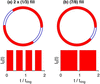
One feature of storage-ring facilities is the temporal structure of the X-ray source on time scales of microseconds and below, owing to the fill pattern of the electron bunches in the accelerator (Cammarata et al., 2009) (see Fig. 1). The fill pattern, and its effect on time correlation functions, has typically been observed using fast single-pixel detectors such as avalanche diodes (Holldack et al., 2007; Lee et al., 2022; Brosi et al., 2025). This periodic time structure is now observable using the new event-driven pixel-array detectors, and will introduce large features into the time correlation functions obtained during high resolution XPCS measurements. The goal of this report is to show how to measure the time correlations introduced by storage-ring sources, and how to remove them from XPCS data.

Figure 1 Schematics of non-uniform electron bunch fill patterns in a storage ring, showing the partial filling of RF `buckets' that produces time structure in the X-ray source. Parts (a) and (b) correspond to the 2 × (1/3) and (7/8) fill patterns, respectively. The cycle time of electrons in the ESRF storage ring is tring = 2.8152 µs.

Initial XPCS experiments in the nanosecond regime have also been performed with very-high-speed framing detectors, which record sequences of complete images (Jo et al., 2021). Event-driven detectors promise to greatly accelerate this progress, because of their unlimited range of lag times, small pixel size, and low cost (Chushkin et al., 2025). The methods developed here can also be applied to XPCS data from framing detectors when the source time structure is resolved.

In this paper, we first discuss the separation of source, detector, and sample contributions to the observed time correlation function g⁽²⁾. We show experimental results for the source contribution, for different non-uniform fill patterns. We then demonstrate that normalization of the observed g⁽²⁾ by the source and detector contributions results in the sample contribution, for both static and dynamic samples. This allows extraction of diffusion relaxation times down to 1 µs and below from a nanoparticle colloid. Finally we discuss the implications of this correction method to allow using standard fill patterns for high-speed XPCS. While we verify the normalization method using XPCS data from an isotropic sample with simple dynamics taken in the small-angle scattering geometry, the same methodology can be applied to XPCS data from other geometries or with more complex dynamics. Likewise, while the verification uses data from some specific fill patterns, the method applies to any fill pattern.

2. Combined dynamics of source and sample

One can write the time dependence of the measured signal in a detector pixel corresponding to a scattering wavevector q as

where I₀(t) is the time-dependent intensity of the source and R(q, t) is the instantaneous speckle pattern produced by the sample (i.e. fraction of intensity into that pixel).

2.1. Autocorrelation function

The fluctuations in the intensity in a given pixel I_p(t) can be characterized by the time autocorrelation function (ACF) for the wavevector q (Shpyrko, 2014),

where Δt is the lag time and 〈…〉 is an ensemble average.

The goal of XPCS measurements is to obtain the fluctuations in the speckle pattern from the sample R(q, t), which can be characterized by

A key aspect of our analysis is the presumption that the dynamics from the source and sample are uncorrelated. This will be valid unless the source intensity is sufficiently strong to drive oscillations in the sample structure on the time scale of the source variations (e.g. microseconds). Typical equilibrium XPCS studies are far from this condition. Since the dynamics from the source and the sample are uncorrelated, we have 〈I_p(t) I_p(t + Δt)〉 = 〈I₀(t) I₀(t + Δt)〉〈R(q, t) R(q, t + Δt)〉, and the correlation function for the observed intensity I_p(t) simply factors into the product of those for the source and the sample,

where fluctuations in the source intensity are characterized by

and we have also included a factor to model any effects introduced by the detector, such as the effect of detector dead time (discussed in Section 5.1).

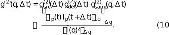
Thus according to equation (4) we should be able to divide the observed ACF g⁽²⁾(q, Δt) by the contributions from the source fill pattern and the detector to obtain the contribution from the sample dynamics. We demonstrate this using measurements of and .

2.2. Ensemble average

A central aspect of XPCS analysis is the method used to obtain the ensemble average 〈…〉 needed in the calculation of g⁽²⁾. For a dynamic sample, where the measurement time is much longer than the fluctuation relaxation time, an average over time t can be used for the ensemble average. To obtain the speckle contrast of a static sample, or when additional averaging is needed to improve statistics, an average over equivalent pixels on the detector is also typically used. For an isotropic sample, g⁽²⁾ depends only on the wavevector magnitude q ≡ |q|, and all pixels at fixed q are equivalent. In the small-angle scattering geometry, the average can be over the azimuthal angle ϕ of a circle on the detector with pixels at fixed q, and equation (2) can be written as

where 〈…〉_t,ϕ is the average over time and ϕ, and the average scattering is ≡ 〈I_p〉_t,ϕ.

As in typical small-angle XPCS analysis, we take averages over pixels falling within an annulus on the detector having an average wavenumber and a finite width Δq. This gives a quantity

where 〈…〉_Δq is the average over the q values within the annulus. A correction can be made for the error that this introduces by assuming that the numerator and denominator of equation (6) both vary with q by the same factor within the annulus, and their ratio is relatively constant. In this case we can write

which gives

We can thus relate to the pixel intensities by

2.3. Cross-correlation function

The time cross-correlation function (CCF) between two neighboring pixels can be useful because it eliminates the detector dead time limitation for fast correlations (Chushkin et al., 2025). It can be written as

where p + Δ indicates a neighbor of pixel p. Here in the denominator we neglect the small difference in q of the neighboring pixels. In this case the CCF of the speckle pattern from the sample is

where q′ corresponds to the neighboring pixel. As discussed in Section 3, this will typically have a lower contrast than the ACF, but should have the same dynamics. We can follow the same analysis given above for the ACF to relate to the pixel intensities,

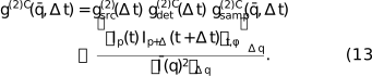
As we shall see in Section 5.1, the contribution of the detector to the CCF, , can differ from its contribution to the ACF, .

3. Experimental setup

The experiments were carried out at the European Synchrotron Radiation Facility (ESRF) beamline ID10-COH, after the EBS upgrade (experiment number SC-5691). We used a combination of undulators (two U27 and one U35) to provide maximum coherent flux. The Si (111) monochromator was set to a photon energy of 11.5 keV (λ = 1.078 Å). Focusing was performed using a compound refractive lens transfocator located at 36 m to image the source at the sample position (61 m). The incident beam was then defined by 10 µm × 10 µm slits, 0.765 m upstream of the sample. This gave a typical incident flux of 1.5 × 10¹¹ photons s⁻¹ with no attenuation.

To observe the arrival times of photons with high time and spatial resolution, we employed the TEMPUS detector (Correa et al., 2024). It is based on the Timepix4 chip (Llopart et al., 2022), with (512 × 448) pixels of 55 µm size. The 0.5 mm-thick Si sensor was biased at 100 V, which gave a time-of-arrival resolution of about 70 ns due to the electron drift time in the sensor. The photon threshold was set to 40 mV, and the Krummenacher current was set to 47 nA. The dead time for detecting a second photon in the same pixel was about 500 ns. There was also a small suppression of second photon events lasting about 1 µs (see the discussion in Section 5.1). We used a transmission small-angle scattering geometry with a sample-to-detector distance of 7.06 m.

The ESRF circumference of 843.977 m corresponds to a ring period of t_ring = 2.8152 µs for the circulating relativistic electrons. The ESRF has a harmonic number of 992, i.e. there are 992 oscillations or `buckets' in the 352.37 MHz RF field around the ring that can each contain electron bunches. This gives a spacing of 2.8379 ns between buckets. A 992-bunch uniform fill at ESRF thus gives flashes of X-rays at the bucket period, which is significantly smaller than the time resolution of the detector we used, so the uniform fill acts like a continuous source and thus is the most suited fill pattern for high-speed XPCS. Conversely, non-uniform fill patterns produce time structure that can typically be resolved by the detector. We studied the effects of two non-uniform fill patterns, labeled 2 × (1/3) and (7/8) (see Fig. 1). Each ring period of the 2 × (1/3) fill pattern had two regions of full buckets, each occupying nominally 1/3 of the ring (∼0.94 µs), separated by gaps of ∼0.47 µs. Each ring period of the (7/8) fill pattern had one region of full buckets, occupying nominally 7/8 of the ring (∼2.46 µs), with one gap of ∼0.35 µs. While non-uniform fill patterns are the most common ones used at ESRF, these particular patterns were non-standard ones, used temporarily because of ring vacuum issues.¹

Two samples were studied, a static Vycor porous glass sample of 200 µm thickness with nanoscale structure due to phase separation, and a dynamic colloid sample of nominally 20 nm-diameter silica nanoparticles in water (5 mg ml⁻¹, silanol surface)² in a 2 mm-diameter capillary. Unless otherwise noted, the temperature of the colloid was 22°C, including a +2°C offset from the temperature control setpoint due to estimated heating of the sample by the unattenuated beam.

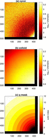
Figs. 2(a) and 2(b) show typical time-averaged small-angle scattering patterns from the Vycor and colloid samples. The Vycor sample gives a ring of scattering with an average radius corresponding to q ≃ 0.023 Å⁻¹, consistent with its phase-separated structure, while the colloid sample gives a peak centered at q = 0, consistent with a spherical nanoparticle form factor. As shown in Fig. S1 of the supporting information, scattering data obtained out to higher q could be fit to give an average particle radius 〈R〉 = 10.9 nm and polydispersity σ_R/〈R〉 = 0.13.

Figure 2 Time-averaged scattering patterns from (a) Vycor and (b) colloid samples, for unattenuated incident beam. (c) Mask used to define annular q ranges for g^(2). All plotted in pixel coordinates. The direct beam is centered at pixel (425, 498).

The TEMPUS detector produces a data stream including arrival times and positions of each detected photon. Since the maximum total count rate of the detector is limited by the transmission speed of this link, only the data from `good' pixels were transmitted; we masked out regions in the direct beam or having significant background scattering from upstream slits, and pixels giving signal when there was no X-ray illumination. The mask used is shown as the black pixels in Fig. 2. For purposes of data storage and processing, this data stream was broken into a sequence of `chunks' of duration 0.1 s. A typical XPCS dataset consisted of many thousands of chunks. Each chunk was processed using an event correlator (Chushkin et al., 2012) to give the ACF of equation (10) for 12 annuli having equally spaced on a logarithmic scale to form a geometric sequence between 0.0039 and 0.0266 Å⁻¹, shown as colored areas in Fig. 2(c). These were calculated for a set of lag times Δt with a linear spacing of 20 ns, and were subsequently binned into a logarithmically spaced set of lag times. The results were then averaged over the many chunks recorded. At this step, chunks with identified data issues could be discarded. In our case, these were a few chunks with detector system communications errors, and a sequence in one dataset with streaky images due to a bubble passing through the beam. A separate paper on the TEMPUS analysis pipeline is in preparation.

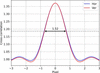
We also calculated the CCF between neighboring pixels (Chushkin et al., 2025), , of equation (13). The CCF allows observation of lag times as small as the 70 ns arrival time resolution of the detector, not limited by the 500 ns dead time of a given pixel (the minimum time lag for a second photon to be detected in the same pixel). When the speckle size is comparable with or larger than a pixel, the CCF is similar to the standard ACF with a reduced contrast. Fig. 3 shows the spatial cross-correlation of the speckle pattern from the static Vycor sample. This gives a speckle size of ∼1.5 pixels and a contrast reduction from ∼37% for the ACF (from the value at pixel 0) to ∼10% for the CCF (from the value at pixel ±1). One can see that if the speckle width decreases below ∼1.5 pixels, the CCF contrast will quickly approach zero. Because of the symmetric scattering geometry and speckle contrast, we averaged the CCFs obtained for neighbors in the vertical and horizontal directions to improve statistics.

Figure 3 Spatial cross-correlation of the time-averaged speckle pattern from Vycor, to determine the speckle size of 1.52 pixels and reduced contrast between neighboring pixels.

4. Determining g_src⁽²⁾(Δt)

4.1. Arrival time distributions

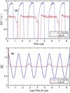
Fig. 4(a) shows typical I₀(t) determined from histograms of the arrival times of photons for the 2 × (1/3) and (7/8) fill patterns, obtained by summing over all pixels and binning over several seconds of data from the Vycor sample. The 70 ns FWHM arrival time resolution of the detector is evident in the rise and fall times surrounding the gaps in the fill patterns. One can see that the actual fill patterns differ from the ideal square waves shown schematically in Fig. 1; the intensity during the region of `full' buckets is not constant. Thus the measured gives a better correction factor than the calculated based on an ideal square wave. Calculations of from ideal square waves and comparisons with measurements are given in Section VII of the supporting information.

Figure 4 (a) Measured intensity versus time and (b) source time correlation function for 2 × (1/3) and (7/8) fill patterns.

4.2. Measuring g_src⁽²⁾(Δt)

Because the contribution from the time structure of the source affects all pixels in the scattering patterns, it is unnecessary to have a separate fast detector to measure . For an equilibrium sample that is ergodic in the sense that all microstates are simultaneously present in the illuminated volume, the source time dependence I₀(t) can be obtained by summing I_p(t) over a range of q including a large number of speckles, or equivalently including the arrival times of the photons in a large range of pixels, as in Fig. 4(a). Equation (5) can then be used to obtain . (It is more efficient to use a standard intensity correlator rather than an event correlator for this high summed intensity.) It is not necessary to use a static sample which introduces no dynamics if the intensity in many speckles is summed, since the contribution from any dynamics in an ergodic equilibrium sample will be negligible. Thus the needed can be obtained from the same sample and dataset used to obtain by using I_p summed over all pixels in each annulus. (The results for each annulus should be equivalent.) If the XPCS sample is not ergodic, a different equilibrium or static sample can be used. However, an advantage of using the calculated from the same dataset for normalization is that this will avoid errors from any changes to the fill pattern that may occur during the time period between samples. Fig. S12 in the supporting information shows how the measured for the same fill pattern at different times can change. Measured from the Vycor sample for the two fill patterns are shown in Fig. 4(b). The amplitude of is smaller for the (7/8) fill than for the 2 × (1/3) fill because of its more uniform I₀(t).

Owing to the strictly periodic nature of the circulating electrons in a storage ring, the intensity correlations extend with constant amplitude to arbitrarily long lag times. Typical XPCS data analysis uses logarithmically spaced lag time bins, which average over larger ranges of Δt at larger Δt, gradually smoothing out the structure in . Logarithmically binned are shown in Figs. 5(a) and 6(a). While the amplitude of the binned decreases with increasing Δt, significant amplitude remains out to tens of microseconds lag time. Thus normalization of the measured g⁽²⁾ by is needed whenever the source has a time structure and the detector has sufficient time resolution to record it.

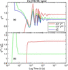
Figure 5 (a) Measured ACF, CCF, and from a static Vycor sample for the 2 × (1/3) fill pattern. (b) Ratios of the ACF and CCF to .

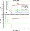
Figure 6 (a) Measured ACF, CCF, and from a static Vycor sample for the (7/8) fill pattern. (b) Ratios of the ACF and CCF to .

5. Normalizing g⁽²⁾(Δt)

5.1. Results: static sample

For a static sample, the lag time dependence of g⁽²⁾(Δt) should be given solely by those of the source and detector. Fig. 5(a) compares the ACF and CCF results for the Vycor sample and the 2 × (1/3) fill pattern, obtained using equations (10) and (13), to the measured of equation (5), all averaged over the region of more intense scattering (q bins 9 to 11, 0.015 Å⁻¹ < q < 0.025 Å⁻¹). The ratios are shown in Fig. 5(b), which represent measurements of the detector contributions and and the speckle contrast. Fig. 6 shows the corresponding results for the static Vycor sample measured using the (7/8) fill pattern.

For both fill patterns, the main lag-time structure in both the ACF and CCF corresponds to . The valid ACF extends to lag times down to ∼500 ns, corresponding to the dead time of a pixel, while the valid CCF extends down to lag times of ∼80 ns, corresponding to the photon arrival time resolution. Above these limits, the CCF ratio is independent of Δt, while the ACF ratio shows a slight dependence on Δt.

We attribute the small dependence of the ACF on Δt to an artifact in the detector electronics where the effective photon threshold for the second photon is raised for a short time after the arrival of the first photon in the same pixel, because of an undershoot in the preamplifier output (Sune et al., 2024). This reduces the probability of detecting the second photon by a small amount, reducing g⁽²⁾(Δt). Such an effect would not be present in the CCF, consistent with our observation. Since we expect the correlation function for the static sample to be a constant, = 1 + β₀, independent of Δt, we have fit the ACF ratios for Δt > 500 ns to the form

For the 2 × (1/3) fill pattern we obtain β₀ = 0.370, δ = −0.0125, and τ_det = 13 µs, while for the (7/8) fill pattern we obtain β₀ = 0.377, δ = −0.0128, and τ_det = 12 µs. The average values of the CCF ratios for Δt > 80 ns give 1 + = 1.095 for the 2 × (1/3) fill pattern and = 1.098 for the (7/8) fill pattern.

In summary, the normalization of the observed g⁽²⁾(Δt) by from equation (5) is very successful in removing the strong oscillations due to the source time structure, and even reveals a weak dependence of the ACF on lag time which we attribute to a detector artifact.

5.2. Results: dynamic sample

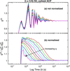
We now turn to normalization of the time structure produced by the fill pattern in the data from the dynamic colloid sample. Figs. 7–10 illustrate the importance of normalizing out the time structure produced by the fill pattern. Fig. 7(a) shows the ACF at various for the colloid sample measured with the 2 × (1/3) fill pattern, without any normalization. (We analyze data only from the first 11 q bins, since the data for q bin 12 are too noisy.) The lag time dependence is dominated by the strong structure from the fill pattern, which is similar to that shown in Fig. 5(a). Fig. 7(b) shows the values normalized by the measured for each q bin, as well as by the weak effect of obtained from the fit to the Vycor ACF data, equation (14). This normalization has successfully removed even the very large amplitude structure produced by the 2 × (1/3) fill pattern.

Figure 7 Measured ACF g^(2) from the dynamic colloid sample using the 2 × (1/3) fill pattern. (a) Not normalized; (b) normalized to and .

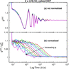
Figure 8 Measured CCF g^(2)C from the dynamic colloid sample using the 2 × (1/3) fill pattern. (a) Not normalized; (b) normalized to .

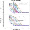
Figure 9 Measured ACF g^(2) from the dynamic colloid sample using the (7/8) fill pattern. (a) Not normalized; (b) normalized to and .

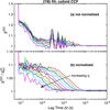
Figure 10 Measured CCF g^(2)C from the dynamic colloid sample using the (7/8) fill pattern. (a) Not normalized; (b) normalized to .

Fig. 8 shows the equivalent results for the CCF function g^(2)C of the colloid sample with the 2 × (1/3) fill pattern. In this case we do not include in the normalization, since the Vycor CCF data indicate that it is negligible. Compared with the ACF results, the valid values extend to lower lag times, and the contrast is smaller, as expected. Thus the correction for the source time structure is even more important for the CCF.

Figs. 9 and 10 show the results obtained for the colloid sample using the (7/8) fill pattern. While the source time correlations introduced from this fill pattern have a lower amplitude than those from the 2 × (1/3) fill pattern, it is still important to remove them, especially for the CCF data. The normalization scheme shown does an excellent job.

As a check, we also acquired ACF and CCF data from the colloid using the ESRF 992-bunch uniform fill mode (see Figs. S4–S6 of the supporting information). As expected, the source contribution calculated from these data using equation (5) is virtually constant, and the primary correction needed for the ACF is .

5.3. Fits to obtain relaxation times

The sample correlation functions obtained after correcting the observed correlation functions for the source and detector can be analyzed to characterize the underlying dynamics in the sample. In the case of colloidal nanoparticles, we expect the dynamics to be dominated by the diffusion of the particles. For a monodisperse colloid of equal size particles, we expect simple exponential behavior of the correlation function at each ,

where B is a baseline near unity, the relaxation time τ(q) is related to the nanoparticle diffusivity D by

and the contrast β can also have a q dependence related to variation of the resolution of the speckle pattern with scattering angle.

When the relaxation time is much larger than the minimum observable lag time , but much smaller than the maximum observable lag time , it is typically straightforward to fit at each to obtain , , and . At Δt ≫ τ, → B, while, at Δt << τ, → B + β, and τ is determined by the lag time at which transitions between these limits.

For the current data this works reasonably well for the CCFs, which have a minimum lag time Δt_min ≃ 80 ns. However, to obtain relaxation times from the ACFs at the higher values, where ≃ 500 ns is not much smaller than τ, it is important to know and fit only two parameters, and . For this purpose we use a functional form based on an approximate analysis of path length distributions, given by

where β₀ is the contrast at q = 0 determined by the coherence of the illumination and the resolution of the detector, fit as a single parameter for all , and most of the other values are known: d = 2 mm is the sample thickness, b = 10 µm is the beam-defining aperture size, R = 7.06 m is the sample-to-detector distance, p = 55 µm is the pixel size, and λ = 1.078 Å is the X-ray wavelength. The parameter f = 1.7 is a factor that we have determined to give the best description of the obtained by fitting the CCF, as shown in Figs. S10 and S11 of the supporting information. This functional form captures the q dependence of β that arises from a relatively thick sample, but neglects the effects of incoherent background on β and B since the samples considered here scatter strongly. It also neglects any difference in the effect of speckle size on the CCF and ACF contrast.

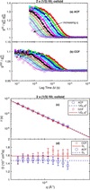
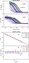
We fit both the ACFs and CCFs of the sample using equations (15)–(17), with fit parameters and for each q region and an overall contrast at q = 0 of β₀. Figs. 11 and 12 show the results for the data taken using the 2 × (1/3) and (7/8) fill patterns, respectively. Values and uncertainties from the fits are listed in Tables S1 and S2 in the supporting information. In all cases, the single exponential function gives a good fit, with τ(q) values that agree reasonably well between the ACF and CCF data. The τ(q) values follow equation (16) to a good approximation, corresponding to a simple diffusive process. Panels (d) of the figures show the diffusivities calculated from each τ point using equation (16), which allows the relative uncertainties arising from the τ values to be seen more easily. The mean diffusivities obtained by fitting the τ(q) values are shown as horizontal lines with values given in Table 1. Values of τ are consistently slightly smaller for the CCF data than the ACF data, resulting in slightly larger extracted diffusivities.

Table 1
Diffusivities and hydrodynamic radii with statistical errors (1σ) for the colloid sample obtained from fits to τ(q) for the ACF and CCF

Fill pattern	T (°C)	DACF (10^−7 cm^2 s^−1)	DCCF (10^−7 cm^2 s^−1)	η(T) (10^−2 poise)	(nm)	(nm)
2 × (1/3)	22	1.47 ± 0.03	1.58 ± 0.03	0.954	15.4 ± 0.3	14.3 ± 0.3
(7/8)	22	1.49 ± 0.02	1.58 ± 0.03	0.954	15.2 ± 0.2	14.4 ± 0.2
Uniform	22	1.54 ± 0.01	1.59 ± 0.01	0.954	14.7 ± 0.1	14.3 ± 0.1
2 × (1/3)	30	1.88 ± 0.04	1.96 ± 0.04	0.797	14.8 ± 0.3	14.2 ± 0.3

Figure 11 Curves show fits of equation (15) to the normalized g^(2) at each wavenumber for the colloid obtained using the 2 × (1/3) fill pattern, for (a) ACF and (b) CCF data (symbols). (c) Symbols show relaxation times as a function of q from the fits to ACF and CCF. Lines show best fits of nanoparticle diffusivity. (d) Data from (c) replotted as D = (τq^2)^−1 versus q.

Figure 12 Curves show fits of equation (15) to the normalized g^(2) at each wavenumber for the colloid obtained using the (7/8) fill pattern, for (a) ACF and (b) CCF data (symbols). (c) Symbols show relaxation times as a function of q from the fits to ACF and CCF. Lines show best fits of nanoparticle diffusivity. (d) Data from (c) replotted as D = (τq^2)^−1 versus q.

Similar fits to ACF and CCF data for the colloid obtained using the ESRF uniform fill give reasonably consistent results (see Fig. S6). We also measured the colloid at 30°C using the 2 × (1/3) fill, and found smaller relaxation times as expected (see Figs. S7–S9). The diffusivity values from these datasets are also listed for comparison in Table 1.

The Stokes–Einstein relation gives the particle diffusivity in terms of the liquid viscosity η as

where R_h is the particle hydrodynamic radius. Using the viscosities of pure water at 22 and 30°C, we can calculate R_h from each of the diffusivities, giving the values shown in Table 1. The values of R_h obtained for the two temperatures are consistent, indicating that the difference in diffusivity arises from the difference in viscosity.

The hydrodynamic radius R_h tends to give more weight to the larger nanoparticles in the size distribution. For the Schulz distribution (Aragón & Pecora, 1976) used in the fit to the time-average scattering pattern, Fig. S1, one can obtain the hydrodynamic radius as (Roosen-Runge et al., 2020) R_h = 〈R〉 [1 + 5(σ_R/〈R〉)²] = 11.8 ± 1.5 nm. Given the uncertainties in the size distribution and the impurities and thus the viscosity of the liquid, this is satisfactory agreement with the values in Table 1.

6. Conclusions

Now that event-driven pixel-array detectors such as TEMPUS (Correa et al., 2024) can resolve the time structure of storage-ring sources of synchrotron radiation, fill patterns can contribute to the observed time correlation functions in XPCS. Because the sample dynamics are uncorrelated with the source dynamics, the observed g⁽²⁾ is given by the product in equation (4), and we can normalize out the time structure of the source. The contribution from the source, , can be quite strong for non-uniform fill patterns, as shown in Figs. 4–6(a). However, even the large amplitude structure produced by fill patterns such as the 2 × (1/3) can be successfully removed to reveal the sample dynamics, as shown in Figs. 7 and 8. This allows us to observe sample dynamics at lag times as small as Δt_min = 80 ns with the TEMPUS, using the CCF. While a static sample can be used to measure , it can also be obtained directly from the dataset of a dynamic sample, simply by first summing the intensity at each time over a large number of pixels.

By removing the effect of the source from the data of a static sample, Figs. 5(b)–6(b), we also observe a small effect in the ACF that is not present in the CCF, which we attribute to a detector artifact (Sune et al., 2024). Like the source effect, this can be measured and normalized out of the ACF according to equation (4).

We demonstrate the normalization method to remove the source and detector dynamics using XPCS data from an isotropic sample with simple diffusive dynamics in the small-angle scattering geometry. However, the method does not depend on the geometry or sample dynamics, and can also be used for wide-angle XPCS, for anisotropic samples, and for complex sample dynamics. Aspects of the analysis specific to the geometry [choice of equivalent pixels on the detector for averaging g⁽²⁾ and calculation of the speckle contrast β(q)] or sample dynamics [choice of an expression for τ(q)] would need to be modified as appropriate.

To extract relaxation times at the highest feasible q values, where is not much smaller than τ, it is important to know the contrast β and how it varies with q, which may differ for ACF and CCF if the speckle size varies with q. This could be characterized using a (relatively) static sample having the same thickness and under the same illumination as the dynamic sample. Lacking such a characterization in the present study, we have simply assumed that the speckle size is independent of q and used the same functional form for β(q), equation (17), for both the ACF and CCF. The small but systematic difference in the relaxation times obtained from the ACF and CCF, shown in Figs. 11 and 12, may result from violation of this assumption. Since the parameter f in equation (17) was determined from β(q) values for the CCF, it is plausible that the τ and D values from the CCF analysis are more reliable than those from the ACF.

There is a correlation between the value of f used and the values of τ(q) obtained. For example, increasing the value of f from 1.7 to 2.9 (giving an increased ratio of β at high q to low q) typically gives ∼5% smaller τ at high q and ∼1% larger τ at low q, resulting in a ∼2% larger D. If this larger value of f = 2.9 was more appropriate for the ACF data, keeping the same value f = 1.7 for the CCF since it was obtained from the CCF β(q), then it would partly explain the difference in the ACF and CCF τ and D.

While a uniform fill pattern is best suited for high-speed XPCS, it is not always available. Our results show that non-uniform fill patterns can be used with the correction methods outlined in this work, thus greatly expanding the availability of suitable beam time.

We have focused on corrections for non-uniform fill patterns with periods on the microsecond scale because the pulse spacing in the ESRF uniform fill mode (2.84 ns) is much smaller than the detector time resolution. However, the pulse spacing of 76.7 ns in the 48-bunch `timing' mode at the upgraded Advanced Photon Source (APS), which is provided for about half of the beam time, can also be resolved by the TEMPUS. Thus even the 48-bunch fill pattern at APS will produce observable structure in XPCS time correlation functions measured with such detectors, and this can be normalized out by the methods presented here.

Footnotes

‡Current address: Eichrom Technologies, LLC, Lisle, IL, USA.

¹The most commonly used filling pattern at ESRF-EBS is the so-called (7/8) + 1, similar to the described (7/8) mode but with a single intense bunch centered in the (7/8) gap.

²Nanocomposix silica nanospheres, 20 nm [NanoXact, 5 mg ml⁻¹, standard (Silanol), 25 ml, water], https://nanocomposix.com/collections/silica-nanoparticles/products/20-nm-silica-nanospheres.

References

Aragón, S. R. & Pecora, R. (1976). J. Chem. Phys. 64, 2395–2404.
Google Scholar
Ballabriga Sune, R., Bromberger, H., Campbell, M., Llopart Cudie, X., Christodoulou, P., Sriskaran, V. & Tlustos, L. (2024). J. Instrum. 19, C03022.
CrossRef
Brosi, M., Schmand, J., Breunlin, J. & Curbis, F. (2025). J. Instrum. 20, P03011.
Cammarata, M., Eybert, L., Ewald, F., Reichenbach, W., Wulff, M., Anfinrud, P., Schotte, F., Plech, A., Kong, Q., Lorenc, M., Lindenau, B., Räbiger, J. & Polachowski, S. (2009). Rev. Sci. Instrum. 80, 015101.
Web of Science
PubMed
Chen, G., Narayanan, S., Stephenson, G. B., Servis, M. J. & Sankaranarayanan, S. K. R. S. (2025). J. Chem. Theory Comput. 21, 8661–8668.
CAS
Chushkin, Y., Caronna, C. & Madsen, A. (2012). J. Appl. Cryst. 45, 807–813.
IUCr Journals
Chushkin, Y., Correa, J., Ignatenko, A., Pennicard, D., Lange, S., Fridman, S., Karl, S., Senfftleben, B., Lehmkühler, F., Westermeier, F., Graafsma, H. & Cammarata, M. (2025). J. Synchrotron Rad. 32, 1220–1227.
Correa, J., Ignatenko, A., Pennicard, D., Lange, S., Fridman, S., Karl, S., Lohse, L., Senfftleben, B., Sergeev, I., Velten, S., Prajapat, D., Bocklage, L., Bromberger, H., Samartsev, A., Chumakov, A., Rüffer, R., von Zanthier, J., Röhlsberger, R. & Graafsma, H. (2024). J. Synchrotron Rad. 31, 1209–1216.
Holldack, K., v, Hartrott, M., Hoeft, F., Neitzke, O., Bauch, E. & Wahl, M. (2007). Proc. SPIE, 6771, 677118.
Hövelmann, S. C., Lange, J., Ignatenko, A., Marin, D., Besana, E., Ster, S., Beckmann, A., Smoljanin, S., Schmehr, J. & Warias, J. E. (2026). AEON event-driven and frame-based X-ray detector, https://zenodo.org/records/22811176.
Jo, W., Westermeier, F., Rysov, R., Leupold, O., Schulz, F., Tober, S., Markmann, V., Sprung, M., Ricci, A., Laurus, T., Aschkan, A., Klyuev, A., Trunk, U., Graafsma, H., Grübel, G. & Roseker, W. (2021). IUCrJ 8, 124–130.
Lee, S., Kwon, H., Cho, B.-G. & Landahl, E. C. (2022). Appl. Sci. 12, 8886.
Lehmkühler, F., Roseker, W. & Grübel, G. (2021). Appl. Sci. 11, 6179.
Llopart, X., Alozy, J., Ballabriga, R., Campbell, M., Casanova, R., Gromov, V., Heijne, E., Poikela, T., Santin, E., Sriskaran, V., Tlustos, L. & Vitkovskiy, A. (2022). J. Instrum. 17, C01044.
Mohanty, S., Cooper, C. B., Wang, H., Liang, M. & Cai, W. (2022). Modell. Simul. Mater. Sci. Eng. 30, 075004.
Raimondi, P., Benabderrahmane, C., Berkvens, P., Biasci, J. C., Borowiec, P., Bouteille, J.-F., Brochard, T., Brookes, N. B., Carmignani, N., Carver, L. R., Chaize, J.-M., Chavanne, J., Checchia, S., Chushkin, Y., Cianciosi, F., Di Michiel, M., Dimper, R., D'Elia, A., Einfeld, D., Ewald, F., Farvacque, L., Goirand, L., Hardy, L., Jacob, J., Jolly, L., Krisch, M., Le Bec, G., Leconte, I., Liuzzo, S. M., Maccarrone, C., Marchial, T., Martin, D., Mezouar, M., Nevo, C., Perron, T., Plouviez, E., Reichert, H., Renaud, P., Revol, J.-L., Roche, B., Scheidt, K.-B., Serriere, V., Sette, F., Susini, J., Torino, L., Versteegen, R., White, S. & Zontone, F. (2023). Commun. Phys. 6, 82.
Roosen-Runge, F., Gulotta, A., Bucciarelli, S., Casal-Dujat, L., Garting, T., Skar-Gislinge, N., Obiols-Rabasa, M., Farago, B., Zaccarelli, E., Schurtenberger, P. & Stradner, A. (2020). Biophys. J. 119, 2483–2496.
Roseker, W., Hruszkewycz, S., Lehmkühler, F., Walther, M., Schulte-Schrepping, H., Lee, S., Osaka, T., Strüder, L., Hartmann, R., Sikorski, M., Song, S., Robert, A., Fuoss, P., Sutton, M., Stephenson, G. & Grübel, G. (2018). Nat. Commun. 9, 1704.
Schoenlein, R. W., Boutet, S., Minitti, M. P. & Dunne, A. (2017). Appl. Sci. 7, 850.
Shi, X., Lin, Y.-C., Zhao, J., Toellner, T., Hu, M. Y., Seifert, S., Lee, B., Grizolli, W., Wojcik, M. J., Rebuffi, L., Assoufid, L. & Sajaev, V. (2025). J. Synchrotron Rad. 32, 1152–1161.
Shpyrko, O. G. (2014). J. Synchrotron Rad. 21, 1057–1064.
Striker, N. N., Schulz, F., Goy, C., Correa, J., Simancas, A., Dallari, F., Marzi, D., Gautam, R. P., Arauz-Moreno, C., Bauer, R. P. C., Chèvremont, W., Cammarata, M., Graafsma, H., Caupin, F. & Lehmkühler, F. (2026). Mater. Adv. 7, 5065–5074.
Sun, Y., Carini, G., Chollet, M., Decker, F.-J., Dunne, M., Fuoss, P., Hruszkewycz, S. O., Lane, T. J., Nakahara, K., Nelson, S., Robert, A., Sato, T., Song, S., Stephenson, G. B., Sutton, M., Van Driel, T. B., Weninger, C. & Zhu, D. (2021). Phys. Rev. Lett. 127, 058001.
Sun, Y., Dunne, M., Fuoss, P., Robert, A., Zhu, D., Osaka, T., Yabashi, M. & Sutton, M. (2020). Phys. Rev. Res. 2, 023099.
Sundararaman, S., Chakraborty, S., Stephenson, G. B., Servis, M. J. & Sankaranarayanan, S. K. R. S. (2026). J. Chem. Phys. 164, 154901.
Tschentscher, T. (2023). Eur. Phys. J. Plus 138, 274.
Tschentscher, T., Bressler, C., Grünert, J., Madsen, A., Mancuso, A. P., Meyer, M., Scherz, A., Sinn, H. & Zastrau, U. (2017). Appl. Sci. 7, 592.
This is an open-access article distributed under the terms of the Creative Commons Attribution (CC-BY) Licence, which permits unrestricted use, distribution, and reproduction in any medium, provided the original authors and source are cited.