Measurements and scaling of X-ray total scattering from single crystals

Gorfman, S.; Eremenko, M.; Krayzman, V.; Bosak, A.; Zavalij, P.Y.; L., I.

doi:10.1107/S1600576726006187

research papers

JOURNAL OF
APPLIED
CRYSTALLOGRAPHY

ISSN: 1600-5767

Volume 59| Part 4| August 2026| Pages 1224-1237

https://doi.org/10.1107/S1600576726006187

Open

access

Measurements and scaling of X-ray total scattering from single crystals

Semën Gorfman,^a ^* Maksim Eremenko,^b,^c,^d Victor Krayzman,^b Alexei Bosak,^e Peter Y. Zavalij ^f and Igor Levin ^b ^*

^aDepartment of Materials Science and Engineering, Tel Aviv University, Tel Aviv, Israel, ^bMaterials Measurement Science Division, National Institute of Standards and Technology (NIST), Gaithersburg, MD 20899, USA, ^cSpallation Neutron Source, Oak Ridge National Laboratory, Oak Ridge, TN, USA, ^dTheiss Research, La Jolla, CA, USA, ^eEuropean Synchrotron Radiation Facility, Grenoble, France, and ^fDepartment of Chemistry and Biochemistry, University of Maryland, College Park, MD 20742, USA
^*Correspondence e-mail: [email protected], [email protected]

Edited by K. Page, University of Tennessee, USA, and Oak Ridge National Laboratory, USA (Received 23 September 2025; accepted 12 June 2026; online 24 July 2026)

This contribution presents a measurement protocol and a data-reduction workflow for obtaining single-crystal X-ray total-scattering datasets that capture both Bragg-peak and diffuse-scattering intensities on an absolute (electrons² per atom) scale. It demonstrates that the intensity scale factor derived from crystallographic refinements using Bragg peaks is in reasonable agreement with the scale obtained by matching the scattering function, computed via spherical integration of the 3D total-scattering signal, to the theoretical coherent baseline. This baseline is calculated from the Debye–Waller factor. The latter scaling approach can be applied to diffuse scattering without including Bragg peaks. These results lay the groundwork for structural refinements using large atomic configurations while simultaneously fitting Bragg intensities and diffuse scattering from a single crystal. Moreover, with the convergence between the two scaling methods, the Bragg and diffuse components can be obtained from the same total-scattering dataset, as achieved in this work, or measured independently.

Keywords: diffuse scattering; total scattering; intensity scaling; structural refinement.

CCDC reference: 2562362

1. Introduction

X-ray or neutron total scattering performed on powder samples has become a common method for analyzing the local and nanoscale structure in crystalline materials. The total scattering includes Bragg peaks that represent the average periodic atomic arrangement, along with a smoothly varying diffuse background that contains information about locally correlated deviations from this average (Egami & Billinge, 2003 ). The Fourier transform of the total signal produces an atomic pair distribution function (PDF). Since interatomic correlations are often anisotropic, the resulting diffuse scattering is also anisotropic (Welberry, 2010 ). The orientational averaging inherent in powder measurements masks this anisotropy, limiting the amount of information that can be extracted from such data.

Recent results demonstrated that combining one-dimensional (1D) total-scattering data from powders with three-dimensional (3D) diffuse scattering from a single crystal enables recovery of occupational and displacement correlations that would be undetectable from powder data alone (Eremenko et al., 2019 ; Krayzman et al., 2022 ; Eremenko et al., 2025 ). Such combined analysis, while powerful, requires both forms of the same material, assumes identical elemental composition and structure for both samples, and requires coordinating measurements across different facilities and instruments, each of which demands specialized expertise. Measurements under non-ambient conditions introduce complications, as variations in sample size and environment can affect controlled parameters. Therefore, if single crystals are available, it would be advantageous to be able to generate quantitative models of correlated atomic disorder across multiple length scales without requiring powder measurements.

One emerging approach toward this goal is the 3D ΔPDF method (Weber & Simonov, 2012 ), which exploits the Fourier transform of the diffuse intensity with Bragg peaks removed. A 3D ΔPDF exhibits positive and negative peaks at or around locations that correspond to distance vectors connecting different pairs of atoms in the average structure. These peaks reflect deviations from the average probability of finding a specific pair. Analyzing the signs, intensities, locations and shapes of these peaks allows determination of the correlations underlying diffuse scattering. While powerful, existing analysis methods for 3D ΔPDF do not produce fully atomistic structural models that would show explicitly how the local structure evolves into the average.

Another solution could involve measuring both Bragg peaks and diffuse scattering from a single crystal in the same dataset and using it to refine large atomic configurations, similar to the current use of powder total-scattering data with the reverse Monte Carlo (RMC) minimization method (Tucker et al., 2007 ; Eremenko et al., 2017 ; Zhang et al., 2020 ). Such data, potentially augmented by direction-resolved X-ray absorption fine structure (Krayzman et al., 2009 ), can be expected to yield highly detailed structural models. The key experimental hurdle is achieving an adequate signal-to-noise ratio (SNR) for the weak diffuse component while avoiding detector saturation by intense Bragg peaks – a problem that has not been adequately addressed so far. Koch et al. (2021 ) considered various artifacts affecting single-crystal total scattering and developed data-processing protocols to mitigate them. Their focus, however, was on producing an artifact-free diffuse-scattering component, without addressing the accuracy of the Bragg-peak intensities. Moreover, some artifacts, such as blooming, which are relevant for the amorphous silicon area detector used in their study, become less significant for the single-photon-counting hybrid pixel detectors increasingly adopted at synchrotron facilities.

In essence, combining integrated Bragg peak intensities and 3D diffuse scattering from a single crystal in structural refinements does not require both components to be in the same dataset. From a practical standpoint, it would be computationally more effective to introduce them separately, with Bragg peaks included to large momentum transfers to provide sensitivity to atomic probability density distributions, and diffuse intensities over more limited reciprocal-space volumes sufficient to uncover correlations but amenable to fitting using current computing power.

Regardless of the analysis approach, quantitative fitting of diffuse scattering, whether in reciprocal space or after the Fourier transform, requires placing intensities on an absolute scale (e.g. electrons² per atom). When Bragg peaks are acquired alongside the diffuse signal, they can be used to calibrate the scale by performing crystallographic refinements of the average structure. Alternatively, as has been shown recently (Eremenko et al., 2025), one can exploit the asymptotic behavior of the scattering function obtained from the spherically integrated diffuse scattering to set the scale of diffuse scattering without Bragg intensities.

Here, we describe a workflow for collecting single-crystal X-ray total-scattering data using a synchrotron beamline optimized for the detection of weak diffuse scattering. We demonstrate an approach to address detector saturation due to Bragg peaks and to subtract Compton scattering, which contributes significantly to the scattering intensity at large momentum transfers. We further show the convergence of the two methods for scaling the intensity of diffuse scattering outlined above. Our validation of the approach, which relies on the known asymptote of the scattering function, enables robust scaling of single-crystal diffuse intensities, opening the door to a flexible combined analysis of Bragg and diffuse scattering even when these signals are collected on different instruments.

2. Experimental

2.1. Test system

In the absence of reference materials with well established atomic probability density distributions and interatomic correlations, we selected the canonical relaxor ferroelectric PbMg_1/3Nb_2/3O₃ (PMN) (Bokov & Ye, 2006 ) as a test system because of the availability of extensive high-quality experimental data and results of large-box structural refinements from a combined fitting of these datasets (Eremenko et al., 2019). PMN exhibits a relatively simple cubic perovskite average structure, but highly complex nanoscale correlations that generate prominent anisotropic diffuse scattering (e.g. Xu et al., 2004 ). We used single crystals of PMN from our previous studies (Eremenko et al., 2019; Eremenko et al., 2025); the crystals did not display any noticeable radiation damage.

2.2. Synchrotron X-ray total-scattering measurements

X-ray scattering intensity from a PMN single crystal was measured at the diffraction side station of the ID28 beamline of the European Synchrotron Radiation Facility (Girard et al., 2019 ). This station is equipped with a HUBER four-circle goniometer, a PILATUS¹ 1M pixel area detector, and single-crystal X-ray diffractometry tools for crystal preparation and mounting. The measurements were conducted at ambient temperature using X-rays with a wavelength of 0.6968 Å. The approximately cylindrical crystal (∼30 µm in diameter) was glued to a glass needle and mounted on the sample holder. Scattering intensity was recorded in the `continuous' mode, in which the crystal rotates at a constant angular speed around the diffractometer φ axis, integrating the detector images over a $[\Delta \varphi = {0.125^ \circ }]$ rotation step and the exposure time τ = 0.25 s. Full 360° rotations were repeated at four different detector angles, achieving a maximum scattering angle 2θ_max = 107° and momentum transfer Q_max ≈ 14 Å⁻¹. The measurements were performed using six different primary-beam absorbers spanning five orders of magnitude in beam attenuation; for stronger absorbers, the full measurement was repeated two to four times to improve counting statistics. The degree of attenuation of the primary beam was determined for each absorber using a beam monitor. The experiment yields J_lab(x_d, y_d, φ) representing the number of photons accumulated inside the detector pixel x_dy_d during the crystal's rotation over the angular range [φ, φ + Δφ] within the time interval τ and using the primary-beam absorber, corresponding to the beam monitor value B. The beam size of ∼50 × 50 µm was defined by the collimator. To ensure the same crystal volume within the beam throughout the experiment, we performed crystal-position scans after each change in the beam absorber.

Additional measurements without the sample indicated that the air-scattering contribution was of the order of a few percent of the diffuse intensity over the sampled Q-range. This contribution is small compared with other systematic uncertainties in the present scaling procedure. We therefore did not apply an explicit air-scattering correction and treat any residual contribution as part of the overall systematic uncertainty.

We used CrysAlisPro (Meyer, 2015 ) for the initial inspection of the scattering intensity and to determine the orientation matrix. The rest of the data analysis was performed using custom MATLAB scripts that provided the necessary flexibility and self-consistency. These scripts are supplied as supplementary information. The first stage of data processing involved determining the centers of mass of the Bragg reflections and refining the orientation matrices for datasets acquired with different beam absorbers. The differences between the obtained orientation matrices corresponded to the maximum strain 10⁻³ and rotation angle of 0.07°. During this refinement, a cubic lattice constraint was varied along with three Euler angles. Subsequently, we performed the reciprocal space reconstruction (RSR) as described below.

2.3. Laboratory X-ray diffraction measurements

A reference set of Bragg-peak intensities was collected with a Bruker D8 Venture diffractometer, where a small fragment of the PMN crystal, about 0.14 × 0.08 × 0.025 mm, was measured at ambient temperature (298 ± 2 K) using Mo Kα radiation (0.71073 Å). The integrated intensities were obtained in the Bruker APEX5 software and corrected for absorption using SADABS (Krause et al., 2015 ). The minimum and maximum transmission values were 0.121 and 0.266, respectively. The measurements covered the hkl range of −8 ≤ h, k, l ≤ 8 out to Q_max = 12.9 Å⁻¹, yielding a total of 7463 reflections, of which 90 unique reflections (R_int = 0.032, R_sig = 0.0154) were used in the structural analysis.

3. Methodology for processing 3D total-scattering data

Fig. 1 presents a workflow that transforms raw intensities into absolute-scale scattering data. The following sections detail each step.

Figure 1
Workflow for converting raw X-ray scattering intensities into absolute-scale data. The intensity notations correspond to those used in the equations presented in the subsequent sections.

3.1. Reciprocal space reconstruction

The first objective of RSR is to transform the instrument-related coordinates x_d, y_d, φ into the components of the scattering vector Q (Fig. 2) and to convert the measured scattering intensity J_lab(x_d, y_d, φ) into the I(Q_x, Q_y, Q_z) = I_cryst(H, K, L) look-up tables. Here, Q_x, Q_y, Q_z / H, K, L denote the components of the scattering vector in either the Cartesian laboratory e_i or the reciprocal crystallographic $[{\bf a}_i^*]$ coordinate systems (see Appendix A and Fig. 2 for more details) and at zero diffractometer angles:

$[{\bf Q} = {Q_x}{{\bf e}_1} + {Q_y}{{\bf e}_2} + {Q_z}{{\bf e}_3} = 2\pi \left({H{\bf a}_1^* + K{\bf a}_2^* + L{\bf a}_3^*} \right). \eqno(1)]$

Figure 2
Schematic illustration of the diffraction experiment, introducing notations used in the text. The image shows the primary X-ray beam, Cartesian laboratory coordinate system e₁ e₂ (e₃ is defined as their cross product). d₀ and d are the unit vectors defining the direction of the detector normal and the direction from the crystal to the given detector pixel, respectively. The angle between these two vectors is defined as the oblique incidence angle η. D₀ is the distance to the detector plane. x_d, y_d are the unit vectors defining the detector axes. Q and Q′ are the scattering vectors before and after rotation.

The second objective is to correct J_lab(x_d, y_d, φ), enabling its conversion to a form that can be modeled using coherent scattering intensity I_coh(Q), which can be expressed as

$[I_{\rm coh}({\bf Q}) = {1 \over N} \sum \limits_m \sum \limits_n {f_m}f_n^*\exp \left( i{\bf Q \cdot R}_{mn} \right). \eqno(2)]$

Here, N is the total number of atoms in the irradiated volume of the crystal, f_m = f_m(Q) are the atomic scattering factors, and R_mn = R_m − R_n is the vector connecting atoms n and m.

Our RSR implements the necessary data correction and normalization steps according to the kinematical theory of X-ray scattering (Warren, 1990 ; Guinier, 1994 ). The first step applies pixel-by-pixel (polarization, Lorentz and oblique incidence) and flat-field (exposure time τ, primary beam monitor B and the distance to the detector D₀) corrections:

$[J_{\rm lab}^{\prime}\left(x_{\rm d},y_{\rm d},\varphi \right) = J_{\rm lab}\left(x_{\rm d},y_{\rm d},\varphi \right)\,R\left(x_{\rm d},y_{\rm d},\varphi \right). \eqno(3)]$

The correction factor R is introduced as (see Appendix B for more details)

$[R\left(x_{\rm d},y_{\rm d},\varphi \right) = {{D_0^{2}} \over {B\tau \sin ^{2}\!\psi \cos ^{3}\!\eta }}\,\delta V^{*}.\eqno(4)]$

Here, ψ = ψ(x_d, y_d) is the angle between the polarization direction of the primary beam and the propagation direction of the scattered beam and η = η(x_d, y_d) is the oblique incidence angle (Fig. 2). δV* = δV*(x_d, y_d, φ) is the reciprocal space volume covered by the single 3D pixel, which can be calculated from the known functional dependence Q_x, y, z(x, y, φ) (see Appendix A for more details):

$[\delta V^{*} = \left| {{{\partial \left({{Q_x},{Q_y},{Q_z}} \right)} \over {\partial \left({x,y,\varphi } \right)}}} \right|S\,{{\Delta}}\varphi, \eqno(5)]$

where S is the area of the detector pixel.

The next RSR step partitions reciprocal space into fixed-size voxels extending over the ΔH, ΔK and ΔL reciprocal lattice units (r.l.u.) along $[{\bf a}_1^{*},{\bf a}_2^{*},{\bf a}_3^{*}]$ , respectively. We assume that the volume of the voxel is significantly greater than δV*. The reconstruction algorithm converts Q_x, Q_y, Q_z into H, K, L and assigns all measured pixels to their corresponding voxels. At this stage, we also symmetrized the data using the operations of the $[m\bar 3m]$ point group, generating symmetric copies of each pixel in the H, K, L space. This symmetrization naturally compensates for missing intensity values arising from the intermodular gaps of the PILATUS detector and improves the robustness of the diffuse-scattering subtraction procedure.

We then accumulate the volume-average voxel intensities I_cryst(H, K, L) according to

$[I_{\rm cryst}\left(H,K,L \right) = {{\sum J_{\rm lab}^{\prime}\left(x_{\rm d},y_{\rm d},\varphi \right)} \over {\sum \delta V^{*}}}. \eqno(6)]$

Here, both summations are over all pixels that fall into the HKL-based voxel. Appendix B shows that these reconstructed values are related to the scattering amplitude as

$[{I_{{\rm cryst}}}\left({H,K,L} \right) = s\langle{I_{{\rm coh}}}\left({H,K,L} \right)\rangle, \eqno(7)]$

where s is the scaling constant and the average is over the HKL-based voxel. Approaches to determining this constant will be considered in the next sections.

Our RSR procedure enables calculating the standard uncertainties σ(H, K, L) of the I_cryst(H, K, L) values, assuming Poisson counting statistics so that σ²(x_d, y_d, φ) = J_lab(x_d, y_d, φ). Then, according to equations (3) and (6)

$[\sigma ^{2}(H,K,L ) = {{\sum J_{\rm lab}\left(x_{\rm d},y_{\rm d},\varphi \right)R^{2}\left(x_{\rm d},y_{\rm d},\varphi \right)} \over {\left(\sum \delta V^{*} \right)^{2} }}.\eqno(8)]$

3.2. The problem of detector oversaturation

The simultaneous acquisition of both Bragg and diffuse-scattering intensities may lead to saturation artifacts in certain pixels J_lab(x_d, y_d, φ), particularly in the proximity of intense Bragg reflections. Moreover, any departure from the linear response of the detector leads to a systematic underestimation of recorded intensity values. The PILATUS active pixel area detector is known to maintain linearity at a photon count rate below 10⁶ cps. This quantity is defined by the deadtime of the detector. Additionally, a hard cap of 1.5 × 10⁶ counts per pixel per frame is imposed by the dynamic range of the detector. A pixel is therefore considered oversaturated if either of these limits is exceeded.

In our experimental setup, each frame was acquired with a minimum exposure time of 0.25 s. Thus, we conservatively define a threshold of 10⁵ counts per pixel per frame, corresponding to an SNR ∼ 300, as a safe upper limit to ensure unsaturated signal acquisition, assuming that the intensity does not vary significantly within a pixel.

If the latter is true, an intuitive approach to correcting oversaturation is to replace saturated pixels with equivalent ones from the dataset measured using an appropriate absorber. However, this approach is not feasible in practice. First, small discrepancies in the refined orientation matrices during successive measurements lead to different reciprocal space coordinates HKL assigned to the same detector pixel. More importantly, in the vicinity of Bragg peaks, the scattered intensity varies rapidly within a pixel over the rotation interval [φ, φ + Δφ]. As a result, even if the recorded (integrated) pixel intensity remains below the threshold, the instantaneous count rate may exceed the count rate threshold, making it impossible to reliably identify saturated pixels on an individual basis.

For these reasons, we perform the correction at the voxel level rather than for individual pixels. Each voxel represents a volumetric element in reciprocal space that aggregates the intensity contribution of 10³ to 10⁴ pixels. For voxel-based reconstructions, we define a higher saturation threshold corresponding to SNR ∼ 1000, providing a robust criterion for identifying and mitigating saturation.

This approach is well suited for diffuse scattering, where the intensity varies slowly over both pixel and voxel dimensions. By combining datasets collected with different absorbers, we construct a lookup table in which the diffuse component is effectively free from saturation artifacts. Figs. 3 and 4 present the results. Fig. 3 displays the two-dimensional reconstruction of 0KL, 1KL and KKL layers, each integrated over the range of 0.05 r.l.u. Fig. 4 provides additional details on the scattering intensity, including its radial and angular dependence as shown in the intensity profile along the cubic face diagonal direction and the polar plot illustrating the anisotropy of the distribution.

Figure 3
Grayscale maps of 2D reconstructions of X-ray scattering intensity in the (a) 0KL, (b) 1KL and (c) KKL layers obtained from the combined (SNR < 1000) dataset, each integrated over the range of 0.05 r.l.u. The maps reveal both sharp Bragg peaks and strongly anisotropic diffuse scattering. Due to the extremely high and typically oversaturated intensity of the Bragg peaks, the grayscale was clipped at 0.0002 of the maximum intensity to enhance the visibility of the diffuse features.

Figure 4
Details of the diffuse-scattering intensity around the 011 Bragg reflection from the combined dataset (SNR < 1000 criterion). The figure consists of three panels that present complementary aspects of the reconstructed intensity distribution in the 0KL reciprocal lattice plane. (a) Reconstructed 2D intensity map around the Bragg peak, displayed over ±0.5 r.l.u. The red circular dashed region marks the radial zone used for angular averaging, and blue dashed lines indicate the strip used to extract a one-dimensional profile along the diagonal direction. (b) Logarithmic intensity profile along the [0KK] ^* reciprocal direction, averaged over a finite-width strip perpendicular to the path. (c) Polar plot of the angular dependence of the diffuse intensity, extracted from the region shown in (a).

This voxel-level criterion becomes unreliable in the vicinity of Bragg peaks, where the photon flux is highly localized within angular regions much smaller than a voxel. In such cases, saturation cannot be reliably detected from voxel-averaged intensities. Therefore, the procedure described above is applied only to diffuse scattering, while Bragg-peak intensities are treated separately, as described in Section 3.4.

3.3. Placing data on the absolute scale

In traditional crystallographic refinements, the scale factor s_B is treated as an independent variable, obtained by minimizing the difference between $[I_{hkl}^{{\rm obs}}]$ and $[s_{\rm B}I_{hkl}^{\rm calc}]$ . Here, $[I_{hkl}^{\rm obs}]$ is the integrated intensity of the hkl Bragg reflection, and $[I_{hkl}^{\rm calc}]$ is defined according to

$[I_{hkl}^{\rm calc} = {1 \over { N_{\rm u}}}\left| F_{hkl}^{\rm calc} \right|^{2}, \eqno(9)]$

where

$[F_{hkl}^{\rm calc} = \sum \limits_{\mu = 1}^{N_{\rm u}} {f_\mu }{T_\mu }{O_\mu }\exp \left[{2\pi i\left({h{x_\mu } + k{y_\mu } + l{z_\mu }} \right)} \right]. \eqno(10)]$

N_u is the number of atoms in the crystallographic unit cell. $[T_{\mu }]$ are the Debye–Waller factors associated with atomic sites having coordinates $[x_{\mu },y_{\mu },z_{\mu}]$ . $[O_{\mu }]$ are the occupancies of these sites. It is possible to show [see e.g. Warren (1990)] that

$[I_{hkl}^{{\rm calc}} = \int\!\!\int\!\!\int_{hkl} I_{\rm coh} (H,K,L)\ {\rm d}H\ {\rm d}K\ {\rm d}L, \eqno(11)]$

where the integration is carried out over the Bragg peak hkl.

In contrast, refinements based on total-scattering data using large atomic configurations require the experimental data to be on an absolute scale (electrons² per atom) so that no scale factor is involved in the fit. Although the scale factor can, in principle, be treated as a variable, in large-configuration refinements with many degrees of freedom (e.g. RMC-type approaches), it becomes strongly coupled with the amplitudes of occupational and displacement correlations. Diffuse intensities generally scale with the square of these correlation amplitudes. Therefore, fitting procedures such as those involving the RMC method will `use' a scale factor to compensate for correlation strength, potentially leading to significantly biased structural parameters (Eremenko et al., 2019; Eremenko et al., 2025; Krayzman et al., 2022). While physical constraints encoded in the data, such as the decay of correlations with distance, reduce this ambiguity, they are often insufficient to drive the fit to the correct solution. For this reason, placing diffuse-scattering data on an absolute scale prior to refinements provides an important external constraint and improves the reliability of the derived structural information.

If both Bragg and diffuse scattering are measured simultaneously, this issue can be resolved by first performing a conventional crystallographic refinement to determine s_B and subsequently rescaling the entire total-scattering dataset, including its diffuse component. Alternatively, the scattering data can be placed on an absolute scale by exploiting the known asymptotic behavior of the powder scattering function, as suggested by Eremenko et al. (2025). In this approach, the 3D total-scattering data are first spherically averaged and converted into the scattering function, which is then matched to its theoretical baseline calculated from the composition and atomic displacement parameters (U_ij). These parameters need only be known approximately and can be adopted from the literature, if available, or estimated from crystallographic refinements using Bragg intensities, either from the same total-scattering dataset or from a separate experiment. Here, we demonstrate that the two scaling methods converge, yielding similar outcomes.

We first present the scaling approach based on the asymptotic behavior of the powder scattering function. The procedure includes the following steps:

Step 1. Integrating the 3D scattering intensity distribution I_cryst(H, K, L) ≡ I(Q) over all possible crystal orientations to obtain a 1D intensity function I(Q) that would be measured for an equivalent powder specimen:

$[I(Q) = \langle I({\bf Q})\rangle_{|{\bf Q}| = Q}. \eqno(12)]$

In practice, this integration is performed by dividing the Q-range of interest into a finite number of bins and averaging all I(Q) values corresponding to each |Q| within a given bin. Fig. 5 displays the result of such averaging for datasets collected with five different beam absorbers. The graphs are vertically offset for clarity, and the zero level for each graph is indicated by a dashed line and a corresponding label specified on the right-hand side.

Figure 5
I(Q) according to equation (12)

for five absorbers (B1–B5, from bottom to top), vertically offset for clarity. In this series, B1 corresponds to the weakest absorber and B5 to the strongest. Horizontal dashed lines indicate the zero-intensity baseline for each curve. The absorber used for each dataset is indicated on the right. According to equations (3)

, (4)

and (12)

, all intensities are normalized to the beam monitor. The figure illustrates saturation effects in Bragg peaks, which result in underestimated intensities when weaker absorbers are used. It also highlights artifacts in the diffuse background arising from limited counting statistics in measurements with stronger absorbers.

Step 2. Introducing the calculated and observed scattering functions.

The calculated scattering function can be expressed (e.g. Farrow & Billinge, 2009 ) as

$[S^{\rm calc}(Q) = { {I_{\rm coh}(Q) - I_{\rm compt}(Q)} \over {\langle f\rangle^{2}N}} - I_{\rm Laue}(Q). \eqno(13)]$

Here, I_coh(Q) is the spherically averaged coherent scattering intensity, I_compt(Q) represents the inelastic Compton scattering and I_Laue(Q) is the monotonic (Laue) diffuse scattering, which in a multicomponent system is expressed as

$[I_{\rm Laue}(Q) = {{\langle f^{2}\rangle} \over {\langle f \rangle^{2}}} - 1. \eqno(14)]$

We define the observed scattering function S^obs(Q) as

$[S^{\rm obs}(Q) = {s \over {\langle f \rangle ^{2}}}\left[I_{\rm cryst}(Q) - p\,I_{\rm compt}(Q) \right] - I_{\rm Laue}(Q), \eqno(15)]$

where s are p are the scaling coefficients. I_compt(Q) is calculated according to Bikondoa & Carbone (2021 ) as described in Appendix C.

Step 3: Determination of the scale coefficients s and p.

The function S^calc(Q) asymptotically approaches unity at high Q. Thus, s and p can be determined by imposing the same requirement on S^obs(Q). Measurements have to extend to Q values sufficiently large for S(Q) to attain this asymptote – a condition that can be verified by considering the expected baseline of the scattering function, $[S_{\rm base}^{\rm calc}(Q)]$ :

$[S_{\rm base}^{\rm calc}(Q) = 1 - {{\langle (f\,\!T )^{2}\rangle} \over {\langle f \rangle^{2}}}, \eqno(16)]$

where

$[\langle (f\,\!T)^{2}\rangle = {1 \over {N_{\rm u}}} \sum \limits_{\mu = 1}^{N_{\rm u}} {O_\mu }\left({{f_\mu }T_\mu ^{\rm s}} \right)^{2}\quad {\rm and} \quad \langle f\rangle^{2} = \left({{1 \over {N_{\rm u}}} \sum \limits_{\mu = 1}^{N_{\rm u}} O_\mu f} \right)^{2}.\eqno(17)]$

Here, $[T_\mu ^{\rm s} = T_\mu ^{\rm s}(Q) = \exp \left( - {1 \over 2}U_{{\rm iso},\mu}Q^{2} \right)]$ is the orientational average of the generally anisotropic Debye–Waller factor, $[{T_\mu } = {T_\mu }({\bf Q})]$ , and U_iso,μ is the equivalent isotropic atomic displacement parameter for site μ. Calculating $[S_{\rm base}^{\rm calc}(Q)]$ requires U_iso,μ and $[{O_\mu }]$ only. The supporting information for this article includes a script that calculates $[S_{{\rm base}}^{{\rm calc}}(Q),\,]$ given the chemical composition and U_ij tensors.

In our case, the conditions were implemented by selecting all data points with Q > Q_min = 12 Å⁻¹ and using linear regression for matching S^obs(Q) to $[S_{{\rm base}}^{{\rm calc}}(Q)]$ to find s and p. Then, we normalized our reconstructed total intensities per atom according to

$[I^{\rm s}({\bf Q}) \leftarrow s\left[I({\bf Q}) - pI_{\rm compt}(Q) \right]. \eqno(18)]$

Fig. 6 shows the resulting scattering function, determined according to equations (16) and (18). The same figure also shows the baseline $[S_{\rm base}^{\rm calc}(Q)]$ . The interval Q > Q_min which was used for linear regression to obtain s and p is highlighted with a rectangle.

Figure 6
Normalized scattering function S^obs(Q) as defined in equation (15)

, where coefficients s and p were calculated so that the resulting S^obs(Q) asymptotically approaches $[S_{\rm base}^{\rm calc}(Q)]$ at high Q. The rectangle on the right highlights the Q-range that was used to determine these coefficients. The red line shows the baseline, calculated according to equations (16)

and (17)

The relative contribution of Compton scattering to the total intensity can reach ∼50% at Q = 14 Å⁻¹ (as shown in Fig. 9 in Appendix C). Subtracting this parasitic background is essential for the quantitative fitting of diffuse intensities to Q > 5 Å⁻¹.

To assess the effect of the choice of Q_min on s and p, we repeated the procedure for a range of Q_min values between 7 and 12 Å⁻¹, while keeping Q_max fixed. The resulting dependencies s(Q_min) and p(Q_min) are shown in Appendix D. The corresponding variations reflect both the statistical uncertainty in the I(Q) values and the systematic uncertainty associated with the scaling procedure. From the maximum relative deviation of s and p over this Q_min range, we estimate their uncertainties not to exceed 6%, yielding s = 0.034 (2) and p = 43 (3).

3.4. Determining Bragg intensities

The RSR process does not distinguish between Bragg and diffuse scattering. However, combining these signals in a single lookup table poses challenges that must be addressed if fitting this table as a single data set. The difficulty arises because Bragg peaks are typically confined to a single detector pixel and have angular widths that are one to two orders of magnitude smaller than Δφ. As a result, experimental data provide Bragg-peak intensities integrated over the corresponding voxel volumes.

Below, we describe a procedure for extracting observed Bragg intensities $[I_{hkl}^{\rm obs}]$ that can be matched to $[I_{hkl}^{\rm calc}]$ calculated from a structural model according to equations (9) and (10). The first step of the proposed procedure involves subtracting the diffuse-scattering background I₀(H, K, L) from the total reconstructed intensity I_cryst(H, K, L). At this stage, the background intensity I₀(H, K, L) beneath the Bragg reflection is estimated by fitting a 3D pseudo-Voigt function to the portion of I_cryst(H, K, L) located at a distance greater than 0.06 r.l.u. from the peak center. Our use of a 3D pseudo-Voigt function does not represent a physically rigorous model of diffuse scattering. We employ it as a flexible, empirical function to approximate the smooth background intensity, enabling separation of Bragg and diffuse contributions as required to address the goals of this study. The extracted Bragg-peak intensity values were found to be insensitive to small variations in the pseudo-Voigt parameters within the fitting uncertainty. The uncertainty associated with the diffuse-background approximation is therefore implicitly included in the uncertainty assigned to the extracted Bragg-peak intensities and propagates into the final scale-factor determination.

Fig. 7 illustrates this background subtraction procedure. It represents a 3D reconstruction of I_cryst(H, K, L) around the 011 reflection, including the HK, HL, KL projections (integrated along the missing coordinate in the range of 0.05 r.l.u.) and H, K and L intensity profiles (integrated over the two missing coordinates). Each 1D plot also includes its corresponding fitted background profile I₀(H, K, L). Then the observed Bragg intensities are calculated as follows:

$[I_{hkl}^{\rm obs} = {\Delta}H\,{\Delta}K\,{\Delta}L\!\! \sum \limits_{HKL \in hkl}\!\! \left[I_{\rm cryst}^{s}(H,K,L) - I_{0}(H,K,L) \right]. \eqno(19)]$

Here, the product ΔH ΔK ΔL defines the voxel volume. This factor is introduced to account for the reciprocal space integration as defined in equation (11). The summation is performed over those voxels in the reciprocal unit cell centered on the reciprocal lattice node hkl that fall within the range (|H − h|, |K − k|, |L − l|) < 0.5.

Figure 7
The reconstructed intensity $[I^{\rm s} = I_{\rm cryst}^{\rm s}(H,K,L)]$ around the 011 Bragg reflection. The top panels show HK, HL and KL projections, while the bottom panels show the H, K and L dependencies, along with the fitted background curve I₀(H, K, L).

We use equation (19) to generate tables of $[I_{hkl}^{{\rm obs}} \pm \sigma _{hkl}^{{\rm obs}}]$ for each measured reflection and each absorber. We then examine these intensities versus the beam monitor value B. Because the RSR normalizes the intensities by B [equations (3) and (4)], unsaturated reflections are flat with respect to B. In contrast, saturated reflections display underestimated intensities at large B, where the primary beam is more intense.

Fig. 8 plots the examples of $[I_{hkl}^{\rm obs}]$ versus B for three reflection groups: strong (110 and 200), medium (221 and 051) and weak (730 and 028). As expected, strong peaks exhibit reduced intensities at large B due to detector saturation; for these reflections, we select intensities from the datasets recorded with a higher-attenuation absorber. Conversely, weak reflections require higher-flux data to achieve adequate SNR. We automated this reflection choice by inspecting $[I_{hkl}^{{\rm obs}} \pm \sigma _{hkl}^{{\rm obs}}]$ as a function of B using the procedure below. For each reflection, this procedure selects the highest-intensity measurement that is not saturated while maintaining sufficient counting statistics.

Figure 8
Dependence of reflection intensities on the primary-beam monitor value B, shown on a logarithmic scale, for three groups of representative reflections: strong (110, 200), medium (221, 051) and weak (730, 028). Each panel displays the integrated intensity $[I_{hkl}^{{\rm obs}}]$ with error bars as a function of $[{\log _{10}}B]$ . For strong reflections, intensities decrease at higher beam-monitor values due to detector saturation. Conversely, weak reflections exhibit low signal-to-noise ratios at low flux. Red circles indicate the absorber setting automatically selected for each reflection by the procedure used to optimize data quality for structural refinement.

(a) Starting from the weakest absorber B₁, we compare successive intensity values $[I_{n} = I_{hkl}^{\rm obs}(B_{n})]$ and their uncertainties $[\sigma _{n} = \sigma _{hkl}^{\rm obs}(B_{n})]$ .

(b) If the condition I_n+1 − I_n > (σ_n+1 + σ_n) is satisfied, the value I_n is considered affected by saturation and is replaced with I_n+1.

(c) The process is repeated iteratively until no further replacements are required or statistically significant values $[[(I_{n}/\sigma _{n})\, \lt\, 5]]$ are exhausted.

In Fig. 8, red circles mark the absorber selected for each reflection. The intensity values for those voxels in the total-scattering dataset that contain Bragg peaks can now be replaced with their corresponding unsaturated values.

4. Crystallographic refinements

All refinements were performed in ShelXle (Hübschle et al., 2011 ; Sheldrick, 2015 ). We considered two Bragg intensity datasets $[I_{hkl}^{\rm obs}]$ : one from the laboratory instrument, with a proven track record of providing reliable structural models, and another from our synchrotron measurements, with intensities extracted as described in Section 3.4. The initial model assumed a perovskite Pm3m space group with all the atoms residing at the ideal positions: Pb @ 1a 000; Mg and Nb @ 1b ½½½; O @ 3c ½½0. This model produced a poor fit and anomalously large atomic displacement parameter for Pb for both datasets (laboratory data: wR2 ≃ 16%, U_Pb ≃ 0.08 Å²; synchrotron data: wR2 ≃ 20%, U_Pb ≃ 0.08 Å²).

We then considered two models with Pb disordered over multiple sites offset from the ideal central position. One assumed Pb atoms shifted along the 〈100〉 directions (Wyckoff position 6e: x 0 0) and the other assumed Pb atoms shifted along the 〈111〉 directions (Wyckoff position 8g: x x x). Both split-site models produced a significant improvement in fit with similar agreement factors for each dataset. For the laboratory data, wR2 ≈ 7.2% and wR2 ≈ 6.98% for the eight- and six-site Pb models, respectively. Regardless of the displacement directions, the magnitude of the Pb off-centering relative to the centrosymmetric positions was ∼0.28 Å. For the synchrotron data, the agreement factors were considerably worse, with wR2 ≈ 9.2% for both eight-site and six-site models. Refining the Nb fraction ratio using the laboratory data yielded 0.652 (14), which is close to the expected value of 0.667. For the synchrotron data, the refined fraction of Nb deviated significantly from the expected value (i.e. 0.5 instead of 0.667); therefore, in the final refinement, we kept the composition fixed at the stoichiometric value. The six- and eight-site models were indistinguishable, in line with the results reported by Eremenko et al. (2025), who observed the coexistence of both types of Pb displacements.

Despite the significantly poorer agreement factors for the synchrotron data, the structural parameters, including the magnitude of the Pb off-centering and the U_ij values for Mg/Nb and O sites, were similar to those obtained from the laboratory data (Table 1), indicating that the structural parameters, in our case, are robust, even in the presence of apparently larger systematic errors. The presence of larger errors in the synchrotron data was also reflected in the relatively large extinction coefficient (1.34), compared with the much more reasonable value of 0.35 obtained from fitting the laboratory dataset.

Table 1
Comparison of structural refinements for the eight-site and six-site Pb models in PbMg_1/3Nb_2/3O₃ using data from the Bruker D8 Venture diffractometer and the ID28 beamline at ESRF

Space group Pm3m; lattice parameter a = 4.0451 (1) Å. In the eight-site model, Pb atoms occupy x x x positions; in the six-site model, they occupy x 0 0 positions. Atomic displacement parameters U_ij are given in Å²; for Nb and Mg, U is isotropic and constrained to be equal for both species. Values in parentheses represent one standard deviation in the last significant digit, as estimated by ShelXle. For the ID28 refinement, the Nb site fraction was fixed.

Parameter	x_Pb	Nb fraction	U₁₁(Pb)	U₂₃(Pb)	U(Nb)	U₁₁(O)	U₃₃(O)
Eight-site
Bruker	0.0391 (3)	0.652 (14)	0.0228 (9)	−0.0059 (3)	0.0085 (5)	0.011 (2)	0.026 (2)
ID28	0.0391 (4)	0.667	0.0237 (8)	−0.0064 (6)	0.0102 (5)	0.011 (2)	0.028 (2)

Six-site
Bruker	0.0684 (4)	0.652 (14)	0.011 (1)	0.027 (1)	0.0085 (5)	0.010 (2)	0.027 (2)
ID28	0.0694 (8)	0.667	0.013 (1)	0.030 (1)	0.0114 (7)	0.008 (3)	0.030 (4)

5. Scale factor

Given that the synchrotron datasets $[I_{hkl}^{\rm obs}]$ were placed on the absolute scale (per atom), the expected scale factor s_B that matches $[I_{hkl}^{\rm obs}]$ and $[{s_{\rm B}}I_{hkl}^{\rm calc}]$ is 1. Accordingly, the scale factor s_F that matches $[I_{hkl}^{\rm obs}]$ and $[s_{\rm F}\left| F_{hkl}^{\rm calc} \right|^{2}]$ (this is how the scale factor is defined in ShelXle) is expected to be equal to $[N_{\rm u}^{ - 1} = 0.2]$ [equation (9)]. Our refinement yields s_F ≈ 0.35. Despite the ∼1.75-fold difference, we regard the agreement as reasonable given the experimental limitations, the strong scale–extinction correlation and the complexity of data processing. This result validates the scaling procedure based on the asymptotic behavior of the scattering function.

Indeed, while the discrepancy of 1.75× may appear significant, in our experience, allowing the scale factor to vary freely in RMC refinements involving diffuse scattering often yields values that deviate by an order of magnitude or more from the absolute scale. The reason is the intrinsic coupling between scale and correlation amplitudes during fitting, as discussed in Section 3.3. By contrast, a discrepancy of ∼1.75× is likely comparable to the uncertainties arising from the various approximations inherent in the extraction of structural information from diffuse scattering.

In ShelXle refinements, the scale factor is strongly correlated with the extinction coefficient. In our case, for the synchrotron data, the correlation coefficient between these two parameters was ∼0.82. For the laboratory data, it was even larger (∼0.92). Despite this strong correlation, the refinements still show a well defined minimum in the agreement factor (R1), as illustrated in Fig. S1 (supporting information), at the scale value close to the reported ∼0.35. The actual uncertainties in the resulting structural parameters, reflecting the combined effect of multiple error sources, including the scale–extinction correlation, can be assessed from Table 1, which compares refinements of the same model using data collected on different instruments. In the present case, the structural parameters appear to be reasonably robust.

Overall, a separate scaling procedure based on the predicted baseline of the scattering function provides a check on the scale factor, improving the reliability of scaled intensities, both Bragg and diffuse. While using Bragg and diffuse components obtained from the same measurements carries obvious advantages, especially when performing in situ measurements, the availability of a validated scaling procedure just for the diffuse part permits combining Bragg and diffuse datasets measured using different instruments.

6. Summary

We developed a procedure to obtain Bragg and diffuse X-ray scattering intensities from a single 3D dataset. Experimental measurements were performed using a synchrotron beamline optimized for recording weak diffuse scattering. The currently unavoidable detector saturation caused by strong Bragg reflections was addressed by collecting data with a series of absorbers spanning five decades in intensity. We developed robust protocols to identify voxels in the reconstructed 3D intensity distributions that were affected by saturation and replace their intensities with those from datasets collected using the appropriate absorber.

We then compared two scaling methods for relating measured intensities to their absolute-scale (electrons² per atom) theoretical values. The first method uses traditional crystallographic refinements, matching Bragg intensities calculated for the average structure model to the observed values. The second, introduced recently but still unverified, matches the 1D scattering function, calculated as a spherical average of the measured scattered intensities, to a theoretical baseline estimated from the chemical composition and atomic displacement parameters. The latter function has a well established behavior at large momentum transfers, which can be used to scale experimental data; this scaling can be performed on diffuse scattering alone, without including Bragg reflections. The two methods yielded reasonably consistent absolute scales, supporting the use of the calculated scattering-function baseline to scale the diffuse portion of the total signal.

With the ability to scale Bragg peaks and diffuse scattering independently, it is possible to combine these datasets in structural refinements even when they were measured with different instruments. For example, a viable approach would be to collect Bragg data using a laboratory diffractometer and diffuse-scattering data at a synchrotron or in an electron microscope. A capability for such refinements, using a list of observed structure factors and 3D diffuse scattering as input, has been implemented in RMCProfile, and examples will be reported separately.

APPENDIX A

Conversion between the instrumental and scattering vector coordinates

This appendix summarizes the relationship between the components of the scattering vector Q = (Q_x, Q_y, Q_z) and the instrumental coordinates x_d, y_d, φ, ω, χ, where

x_d, y_d are detector-plane coordinates of a given detector pixel,

φ is the crystal rotation angles around the corresponding Eulerian cradle axis,

ω and χ are the other two Eulerian angles (typically held constant during the acquisition).

The scattering vector Q is defined in the laboratory coordinate system corresponding to the diffractometer configuration where all Eulerian angles (ω, χ, φ) are set to zero.

We use the standard definition of the scattering vector:

$[{\bf Q}^{\prime} = {{2\pi } \over \lambda }({\bf e}_{1} + {\bf d}). \eqno(20)]$

Here

λ is the X-ray wavelength,

e₁ is the unit vector pointing from the crystal to the X-ray source,

d is the unit vector pointing from the crystal to the detector pixel.

The vector d = D_xy/D_xy is given by the normalized detector-pixel position vector D_xy:

$[{\bf D}_{xy} = {D_0}{\bf d}_{0} + x{\bf x}_{\rm d} + y{\bf y}_{\rm d}, \eqno(21)]$

where

D₀ is the distance from the sample to the detector plane,

d₀ is the unit vector that is normal to the detector plane,

x_d and y_d are the unit vectors defining the detector axes.

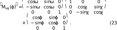
Equations (20) and (21) allow us to calculate the coordinates of the vector $[{\bf Q}^{\prime} = (Q_x^{\prime},Q_y^{\prime},Q_z^{\prime} )]$ . To obtain the corresponding scattering vector in the unrotated laboratory frame, we apply the inverse of the rotation matrix [M_ωχ(φ)]:

$[\left({\matrix{ {{Q_x}} \cr {{Q_y}} \cr {{Q_z}} \cr } } \right) = {\left [{{M_{\omega \chi }}\left(\varphi \right)} \right]^{ - 1}}\left({\matrix{ {Q_x^{\prime}} \cr {Q_y^{\prime}} \cr {Q_z^{\prime}} \cr } } \right). \eqno(22)]$

The total rotation matrix [M_ωχ(φ)], as defined by e.g. Gorfman et al. (2021 ), is the product of three elementary rotations:

$[\eqalignno{\left [M_{\omega \chi }(\varphi) \right] =&\pmatrix{\cos \omega & \sin \omega & 0 \cr -\sin {\omega} & \cos \omega & 0 \cr 0 & 0 &1 } \pmatrix{1 & 0 & 0 \cr 0 & \cos \chi & \sin \chi \cr 0 & -\sin { \chi } &\cos \chi } \cr &\times \pmatrix{ \cos \varphi &\sin \varphi & 0 \cr -\sin { \varphi }&{\cos \varphi } & 0 \cr0 & 0 &1} . & (23)}]$

All the coordinate axes are summarized in Fig. 2.

APPENDIX B

Relationship between measured and theoretical intensities

This appendix summarizes key elements of the kinematical X-ray scattering theory that relate the measured intensity J_lab(x_d, y_d, φ) to the calculated coherent scattering intensity I_coh(Q).

We begin by defining the measured quantity J_lab(x_d, y_d, φ), which represents the number of photons accumulated at the detector pixel (x_d, y_d) during the continuous rotation of the crystal over an angular range [φ, φ + Δφ] and exposure time τ:

$[J_{\rm lab}(x_{\rm d},y_{\rm d},\varphi ) = {\tau \over {\Delta\varphi }} \int \nolimits_{\varphi \,}^{\varphi + {\Delta}\varphi } J_{\rm flux}(x_{\rm d},y_{\rm d},\varphi)\ {\rm d}\varphi. \eqno(24)]$

Here J_flux(x_d, y_d, φ) is the instantaneous photon flux (in photons s⁻¹) arriving at the pixel during the rotation. This flux can be related to the local flux density J_fd(x, y, φ) (in photons s⁻¹ mm⁻²) via integration over the pixel area S, accounting for the oblique incidence angle η (the angle between the scattered ray and the detector normal):

$[J_{\rm flux}\left(x_{\rm d},y_{\rm d},\varphi \right) = \cos \eta \int\!\!\!\int \nolimits_{\rm PIXEL} J_{\rm fd}\left(x,y,\varphi \right)\ {\rm d}x\ {\rm d}y. \eqno(25)]$

According to the kinematical theory of X-ray scattering (Warren, 1990; Guinier, 1994; Als-Nielsen & McMorrow, 2011 ), the local flux density is given by

$[J_{\rm fd}(x,y,\varphi) = J_{0}{{r_{\rm e}^{2}} \over { D^{2}}}P(x,y)\left| A^{\prime}(x,y,\varphi) \right|^{2}. \eqno(26)]$

Here

$[{J_0} = J_0^{\prime}B]$ is the incident beam flux density (measured in photons s⁻¹ mm⁻²). We assume that it is proportional to the reading of the primary beam monitor B with $[J_0^{\prime}]$ being the proportionality factor that remains constant during the experiment.

r_e is the classical electron radius.

D is the sample-to-pixel distance.

P(x, y) = sin²ψ(x, y) is the polarization factor.

A′(x, y, φ) is the scattering amplitude corresponding to detector position (x, y) at rotation angle φ.

To simplify notation, we define the sample-to-detector distance as D₀ = D cos η and re-write (24) as

$[J_{\rm lab}(x_{\rm d}, y_{\rm d}, \varphi) = {J_0}{ {r_{\rm e}^{2}} \over {D^{2}_{0}}} {{\tau} \over {{\Delta\varphi}} } \cos^{3}\eta\, P \!\int\!\!\int\!\!\int\! |A^{\prime}(x,y,\varphi)|^{2}\ {\rm d}x\ {\rm d}y\ {\rm d}\varphi. \eqno(27)]$

Next, we use the functional dependence between the instrumental (x, y, φ) and the scattering vector (Q_x, Q_y, Q_z) in the unrotated reference frame as described in Appendix A as Q(x, y, φ). Substituting A′(x, y, φ) = A(Q_x, Q_y, Q_z), equation (27) becomes

$[J_{\rm lab}(x_{\rm d}, \!y_{\rm d},\! \varphi) = J_{0}{{r_{\rm e}^{2}} \over {D^{2}_{0}}} {\tau \over {{\Delta\varphi}} } \cos^{3}\!\eta\, P \!\!\int\!\!\!\int\!\!\!\int\! |A(Q_{x},Q_{y},Q_{z})|^{2}\,{\rm d}x\,{\rm d}y\,{\rm d}\varphi.\eqno(28)]$

We now introduce the generalized Lorentz factor as the inverse Jacobian determinant:

$[L^{ - 1}\left({x,y,\varphi } \right) = \left| {{{\partial \left({{Q_x},{Q_y},{Q_z}} \right)} \over {\partial \left({x,y,\varphi } \right)}}} \right|, \eqno(29)]$

which allows a change of variables: $[{\rm d}x\ {\rm d}y\ {\rm d}\varphi]$ = $[L(x,y,\varphi)\ {\rm d}{Q_x}\ {\rm d}{Q_y}\ {\rm d}{Q_z}.]$ Substituting this into equation (28), we obtain

$[\eqalignno{J_{\rm lab}(x_{\rm d}, y_{\rm d}, \varphi) = &\,J_{0}{ {r_{\rm e}^{2}} \over {D^{2}_{0}}} {{\tau} \over {{\Delta\varphi}} } \cos^{3}\!\eta LP\cr &\times \int\!\!\int\!\!\int \left|A(Q_{x},\!Q_{y},\!Q_{z})\right|^{2}\ {\rm d}Q_{x}\ {\rm d}Q_{y}\ {\rm d}Q_{z}. &(30)}]$

Although, both the Lorentz factor L and polarization factor P vary across the detector, they can be treated as constant over the small reciprocal-space volume δ V^* covered by the single 3D pixel. This allows an alternative expression for the Lorentz factor in terms of the volume ratios:

$[L(x,y,\varphi ) = {{\Delta\varphi \,S} \over {\delta V^{*}} }\,, \eqno(31)]$

so that equation (30) is transformed into

$[\eqalignno{J_{\rm lab}(x_{\rm d}, y_{\rm d}, \varphi) =\,&J_{0}{ {r_{\rm e}^{2}} \over {D^{2}_{0}}} {S{\tau} \over {\delta V^*}} \cos^{3}\eta\, P\cr &\times \int\!\!\int\!\!\int \left|A(Q_{x},Q_{y},Q_{z})\right|^{2}\ {\rm d}Q_{x}\ {\rm d}Q_{y}\ {\rm d}Q_{z}. &(32)}]$

Applying the multiplicative correction factor as defined in (3) and (4) of the main text,

$[R(x_{\rm d},y_{\rm d},\varphi ) = { {D_0^{2}} \over {B\tau \sin^{2}\!\psi \cos ^{3} \eta }}\,\delta V^{*}, \eqno(33)]$

we obtain the corrected scattering intensity as

$[J_{\rm lab}^{\prime}(x_{\rm d}, y_{\rm d}, \varphi) = R_{0} \int\!\!\int\!\!\int \left|A(Q_{x},Q_{y},Q_{z})\right|^{2}\ {\rm d}Q_{x}\ {\rm d}Q_{y}\ {\rm d}Q_{z}.\eqno(34)]$

Here, R₀ accumulates the factors that remain constant during the experiment:

$[R_{0} = J_0^{\prime}r_{\rm e}^{2}S. \eqno(35)]$

The reconstruction procedure was introduced in the main text: it involves converting the corrected intensity $[J_{\rm lab}^{\prime}\left(x_{\rm d},y_{\rm d},\varphi\right)]$ into I_cryst(H, K, L) as

$[I_{\rm cryst}(H,K,L) = {{\sum J_{\rm lab}^{\prime}\left(x_{\rm d},y_{\rm d},\varphi \right)} \over {\sum \delta V^{*}}},\eqno(36)]$

which means

$[I_{\rm cryst} (H,K,L) = R_{0}\left| A({\bf Q}) \right|^{2}. \eqno(37)]$

Here, the averaging is performed over the reciprocal-space voxel corresponding to the coordinates HKL.

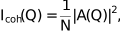
Finally, we recall the standard kinematical theory expression for the scattering amplitude:

$[A({\bf Q}) = \sum \limits_m {f_m}(Q)\exp (i{\bf Q\cdot R}_{m}). \eqno(38)]$

This is directly connected to the definition of the coherent scattering intensity (2)

$[{I_{{\rm coh}}}({\bf Q}) = {1 \over N}{\left| {A({\bf Q})} \right|^2},]$

which leads to equation (7) in the main text:

$[{I_{{\rm cryst}}}\left({H,K,L} \right) = s\langle{I_{{\rm coh}}}\left({H,K,L} \right)\rangle,\quad s = NR_{0}. \eqno(40)]$

APPENDIX C

Compton scattering

The intensity of Compton scattering is calculated as

$[I_{\rm compt}(Q) = K(Q)S_{\rm inc}(Q), \eqno(41)]$

where K(Q) is known as the Klein–Nishina factor:

$[K(Q) = {E^{\prime} \over E}\left({ E \over {E^{\prime}}} + { {E^{\prime}} \over E } - 2\sin ^{2} 2\theta \cos ^{2}\psi \right).\eqno(42)]$

Here, E and E′ are the energies of the incident and incoherently scattered photons, respectively. E′ is determined through

$[{{E} \over {E^{\prime}}} = 1 + {{E} \over {E_{\rm e}}}\left(1 - \cos 2\theta \right) \eqno(43)]$

and E_e = 0.511 MeV is the rest energy of a free electron.

The incoherent scattering function S_inc(Q) is evaluated as an incoherent sum of contributions from all the atoms in the unit cell

$[{S_{\rm inc}}(Q) = \sum \limits_{\mu = 1}^{N_{\rm u}} {O_\mu }\,{s_{{\rm inc},\mu }}(Q),\eqno(44)]$

where the sum runs over N_u atoms in the unit cell, $[{O_\mu }]$ denotes the partial occupancy of the μth atom and s_inc,μ(Q) is the tabulated incoherent scattering factor for the corresponding chemical element (Balyuzi, 1975 ).

Fig. 9 shows the relative contribution of the Compton scattering intensity, defined as I_compt,r(Q) = pI_compt(Q)/I(Q) with the scale factor p determined as described in Section 3.3.

Figure 9
Q dependence of Compton scattering contribution defined as I_compt,r(Q) = pI_compt(Q)/I(Q). The graph shows that at high Q values Compton scattering can contribute significantly — up to 50% to the total scattering.

APPENDIX D

Dependence of the scale factors on Q_min and estimation of their uncertainties

Fig. 10 illustrates how the choice of Q_min affects the resulting scaling coefficients. The corresponding variations reflect both the statistical uncertainty in the I(Q) values and the systematic uncertainty associated with the scaling procedure.

Figure 10
Dependences of the scaling coefficients s and p on Q_min.

Supporting information

CCDC reference: 2562362

Crystal structure: contains datablocks global, I, II, III, IV. DOI: https://doi.org/10.1107/S1600576726006187/pag5004sup1.cif

Structure factors: contains datablock I. DOI: https://doi.org/10.1107/S1600576726006187/pag5004IIsup2.hkl

Supplementary software packages for reciprocal-space intensity reconstruction (MATLAB) and scattering function baseline calculation (Python). DOI: https://doi.org/10.1107/S1600576726006187/pag5004sup3.zip

This supplemental material discusses the correlation between the scale and extinction factors. DOI: https://doi.org/10.1107/S1600576726006187/pag5004sup4.pdf

Computing details top

(I) top

Crystal data top

Mg_0.35Nb_0.65O₃Pb	F(000) = 137
M_r = 324.23	D_x = 8.134 Mg m⁻³
Cubic, Pm3m	Mo Kα radiation, λ = 0.71073 Å
a = 4.0451 (1) Å	µ = 66.23 mm⁻¹
V = 66.19 (1) Å³	T = 298 K
Z = 1	0.14 × 0.08 × 0.03 mm

Data collection top

7463 measured reflections	θ_max = 46.9°, θ_min = 5.0°
90 independent reflections	h = −8→8
90 reflections with I > 2σ(I)	k = −8→8
R_int = 0.077	l = −8→8

Refinement top

Refinement on F²	0 restraints
Least-squares matrix: full	w = 1/[σ²(F_o²) + 0.493P] where P = (F_o² + 2F_c²)/3
R[F² > 2σ(F²)] = 0.025	(Δ/σ)_max < 0.001
wR(F²) = 0.070	Δρ_max = 0.93 e Å⁻³
S = 1.44	Δρ_min = −1.33 e Å⁻³
90 reflections	Extinction correction: SHELXL-2019/2 (Sheldrick 2019), Fc^*=kFc[1+0.001xFc²λ³/sin(2θ)]^-1/4
9 parameters	Extinction coefficient: 0.36 (4)

Special details top

Geometry. All esds (except the esd in the dihedral angle between two l.s. planes) are estimated using the full covariance matrix. The cell esds are taken into account individually in the estimation of esds in distances, angles and torsion angles; correlations between esds in cell parameters are only used when they are defined by crystal symmetry. An approximate (isotropic) treatment of cell esds is used for estimating esds involving l.s. planes.

Fractional atomic coordinates and isotropic or equivalent isotropic displacement parameters (Å²) top

	x	y	z	U_iso*/U_eq	Occ. (<1)
Pb1	0.0684 (4)	0.000000	0.000000	0.0221 (8)	0.1666
Nb2	0.500000	0.500000	0.500000	0.0085 (5)	0.650 (14)
Mg2	0.500000	0.500000	0.500000	0.0085 (5)	0.350 (14)
O3	0.000000	0.500000	0.500000	0.0212 (13)

Atomic displacement parameters (Å²) top

	U¹¹	U²²	U³³	U¹²	U¹³	U²³
Pb1	0.0112 (7)	0.0275 (9)	0.0275 (9)	0.000	0.000	0.000
Nb2	0.0085 (5)	0.0085 (5)	0.0085 (5)	0.000	0.000	0.000
Mg2	0.0085 (5)	0.0085 (5)	0.0085 (5)	0.000	0.000	0.000
O3	0.011 (2)	0.027 (2)	0.027 (2)	0.000	0.000	0.000

Geometric parameters (Å, º) top

Pb1—Pb1ⁱ	0.391 (3)	Nb2—O3^ix	2.0226 (1)
Pb1—Pb1ⁱⁱ	0.391 (3)	Nb2—O3ⁱⁱⁱ	2.0226 (1)
Pb1—Pb1ⁱⁱⁱ	0.391 (3)	Nb2—O3	2.0226 (1)
Pb1—Pb1^iv	0.391 (3)	Nb2—O3^x	2.0226 (1)
Pb1—Pb1^v	0.554 (4)	Nb2—O3^iv	2.0226 (1)
Pb1—O3ⁱⁱⁱ	2.6718 (12)	Nb2—O3^xi	2.0226 (1)
Pb1—O3^iv	2.6718 (12)	Mg2—O3^ix	2.0226 (1)
Pb1—O3^vi	2.6718 (12)	Mg2—O3ⁱⁱⁱ	2.0226 (1)
Pb1—O3^vii	2.6718 (12)	Mg2—O3	2.0226 (1)
Pb1—Mg2	3.3510 (9)	Mg2—O3^x	2.0226 (1)
Pb1—Nb2	3.3510 (9)	Mg2—O3^iv	2.0226 (1)
Pb1—Nb2^viii	3.3510 (9)	Mg2—O3^xi	2.0226 (1)

Pb1ⁱ—Pb1—Pb1ⁱⁱ	60.0	Pb1—Nb2—Pb1^xiv	173.30 (5)
Pb1ⁱ—Pb1—Pb1ⁱⁱⁱ	90.0	Pb1^xii—Nb2—Pb1^xiv	6.70 (5)
Pb1ⁱⁱ—Pb1—Pb1ⁱⁱⁱ	60.0	Pb1ⁱⁱⁱ—Nb2—Pb1^xiv	173.30 (4)
Pb1ⁱ—Pb1—Pb1^iv	60.0	Pb1^xiii—Nb2—Pb1^xiv	6.70 (4)
Pb1ⁱⁱ—Pb1—Pb1^iv	90.0	Pb1^iv—Nb2—Pb1^xiv	180.0
Pb1ⁱⁱⁱ—Pb1—Pb1^iv	60.0	O3^ix—Mg2—O3ⁱⁱⁱ	180.0
Pb1ⁱ—Pb1—Pb1^v	45.0	O3^ix—Mg2—O3	90.0
Pb1ⁱⁱ—Pb1—Pb1^v	45.0	O3ⁱⁱⁱ—Mg2—O3	90.0
Pb1ⁱⁱⁱ—Pb1—Pb1^v	45.0	O3^ix—Mg2—O3^x	90.0
Pb1^iv—Pb1—Pb1^v	45.0	O3ⁱⁱⁱ—Mg2—O3^x	90.0
Pb1ⁱ—Pb1—O3ⁱⁱⁱ	117.518 (17)	O3—Mg2—O3^x	90.0
Pb1ⁱⁱ—Pb1—O3ⁱⁱⁱ	175.80 (3)	O3^ix—Mg2—O3^iv	90.0
Pb1ⁱⁱⁱ—Pb1—O3ⁱⁱⁱ	117.518 (17)	O3ⁱⁱⁱ—Mg2—O3^iv	90.0
Pb1^iv—Pb1—O3ⁱⁱⁱ	85.80 (3)	O3—Mg2—O3^iv	90.0
Pb1^v—Pb1—O3ⁱⁱⁱ	130.80 (3)	O3^x—Mg2—O3^iv	180.0
Pb1ⁱ—Pb1—O3^iv	175.80 (3)	O3^ix—Mg2—O3^xi	90.0
Pb1ⁱⁱ—Pb1—O3^iv	117.518 (17)	O3ⁱⁱⁱ—Mg2—O3^xi	90.0
Pb1ⁱⁱⁱ—Pb1—O3^iv	85.80 (3)	O3—Mg2—O3^xi	180.0
Pb1^iv—Pb1—O3^iv	117.518 (17)	O3^x—Mg2—O3^xi	90.0
Pb1^v—Pb1—O3^iv	130.80 (3)	O3^iv—Mg2—O3^xi	90.0
O3ⁱⁱⁱ—Pb1—O3^iv	64.73 (3)	O3^ix—Mg2—Pb1	127.126 (12)
Pb1ⁱ—Pb1—O3^vi	85.80 (3)	O3ⁱⁱⁱ—Mg2—Pb1	52.874 (12)
Pb1ⁱⁱ—Pb1—O3^vi	117.518 (17)	O3—Mg2—Pb1	58.60 (3)
Pb1ⁱⁱⁱ—Pb1—O3^vi	175.80 (3)	O3^x—Mg2—Pb1	127.126 (12)
Pb1^iv—Pb1—O3^vi	117.518 (17)	O3^iv—Mg2—Pb1	52.874 (12)
Pb1^v—Pb1—O3^vi	130.80 (3)	O3^xi—Mg2—Pb1	121.40 (3)
O3ⁱⁱⁱ—Pb1—O3^vi	64.73 (3)	O3^ix—Mg2—Pb1^xii	58.60 (3)
O3^iv—Pb1—O3^vi	98.40 (6)	O3ⁱⁱⁱ—Mg2—Pb1^xii	121.40 (3)
Pb1ⁱ—Pb1—O3^vii	117.518 (17)	O3—Mg2—Pb1^xii	127.126 (12)
Pb1ⁱⁱ—Pb1—O3^vii	85.80 (3)	O3^x—Mg2—Pb1^xii	52.874 (12)
Pb1ⁱⁱⁱ—Pb1—O3^vii	117.518 (17)	O3^iv—Mg2—Pb1^xii	127.126 (12)
Pb1^iv—Pb1—O3^vii	175.80 (3)	O3^xi—Mg2—Pb1^xii	52.874 (12)
Pb1^v—Pb1—O3^vii	130.80 (3)	Pb1—Mg2—Pb1^xii	173.30 (5)
O3ⁱⁱⁱ—Pb1—O3^vii	98.40 (6)	O3^ix—Mg2—Pb1ⁱⁱⁱ	121.40 (3)
O3^iv—Pb1—O3^vii	64.73 (3)	O3ⁱⁱⁱ—Mg2—Pb1ⁱⁱⁱ	58.60 (3)
O3^vi—Pb1—O3^vii	64.73 (3)	O3—Mg2—Pb1ⁱⁱⁱ	52.874 (12)
Pb1ⁱ—Pb1—Mg2	142.671 (15)	O3^x—Mg2—Pb1ⁱⁱⁱ	127.126 (12)
Pb1ⁱⁱ—Pb1—Mg2	142.671 (15)	O3^iv—Mg2—Pb1ⁱⁱⁱ	52.874 (12)
Pb1ⁱⁱⁱ—Pb1—Mg2	86.65 (2)	O3^xi—Mg2—Pb1ⁱⁱⁱ	127.126 (12)
Pb1^iv—Pb1—Mg2	86.65 (2)	Pb1—Mg2—Pb1ⁱⁱⁱ	6.70 (4)
Pb1^v—Pb1—Mg2	121.40 (3)	Pb1^xii—Mg2—Pb1ⁱⁱⁱ	180.0
O3ⁱⁱⁱ—Pb1—Mg2	37.126 (12)	O3^ix—Mg2—Pb1^xiv	52.874 (12)
O3^iv—Pb1—Mg2	37.126 (12)	O3ⁱⁱⁱ—Mg2—Pb1^xiv	127.126 (12)
O3^vi—Pb1—Mg2	96.69 (4)	O3—Mg2—Pb1^xiv	127.126 (12)
O3^vii—Pb1—Mg2	96.69 (4)	O3^x—Mg2—Pb1^xiv	58.60 (3)
Pb1ⁱ—Pb1—Nb2	142.671 (15)	O3^iv—Mg2—Pb1^xiv	121.40 (3)
Pb1ⁱⁱ—Pb1—Nb2	142.671 (15)	O3^xi—Mg2—Pb1^xiv	52.874 (12)
Pb1ⁱⁱⁱ—Pb1—Nb2	86.65 (2)	Pb1—Mg2—Pb1^xiv	173.30 (5)
Pb1^iv—Pb1—Nb2	86.65 (2)	Pb1^xii—Mg2—Pb1^xiv	6.70 (5)
Pb1^v—Pb1—Nb2	121.40 (3)	Pb1ⁱⁱⁱ—Mg2—Pb1^xiv	173.30 (4)
O3ⁱⁱⁱ—Pb1—Nb2	37.126 (12)	O3^ix—Mg2—Pb1^iv	127.126 (12)
O3^iv—Pb1—Nb2	37.126 (12)	O3ⁱⁱⁱ—Mg2—Pb1^iv	52.874 (12)
O3^vi—Pb1—Nb2	96.69 (4)	O3—Mg2—Pb1^iv	52.874 (12)
O3^vii—Pb1—Nb2	96.69 (4)	O3^x—Mg2—Pb1^iv	121.40 (3)
Mg2—Pb1—Nb2	0.0	O3^iv—Mg2—Pb1^iv	58.60 (3)
Pb1ⁱ—Pb1—Nb2^viii	86.65 (2)	O3^xi—Mg2—Pb1^iv	127.126 (12)
Pb1ⁱⁱ—Pb1—Nb2^viii	86.65 (2)	Pb1—Mg2—Pb1^iv	6.70 (4)
Pb1ⁱⁱⁱ—Pb1—Nb2^viii	142.671 (15)	Pb1^xii—Mg2—Pb1^iv	173.30 (5)
Pb1^iv—Pb1—Nb2^viii	142.671 (15)	Pb1ⁱⁱⁱ—Mg2—Pb1^iv	6.70 (5)
Pb1^v—Pb1—Nb2^viii	121.40 (3)	Pb1^xiv—Mg2—Pb1^iv	180.0
O3ⁱⁱⁱ—Pb1—Nb2^viii	96.69 (4)	O3^ix—Mg2—Pb1^xiii	52.874 (12)
O3^iv—Pb1—Nb2^viii	96.69 (4)	O3ⁱⁱⁱ—Mg2—Pb1^xiii	127.126 (12)
O3^vi—Pb1—Nb2^viii	37.126 (12)	O3—Mg2—Pb1^xiii	121.40 (3)
O3^vii—Pb1—Nb2^viii	37.126 (12)	O3^x—Mg2—Pb1^xiii	52.874 (12)
Mg2—Pb1—Nb2^viii	117.21 (5)	O3^iv—Mg2—Pb1^xiii	127.126 (12)
Nb2—Pb1—Nb2^viii	117.21 (5)	O3^xi—Mg2—Pb1^xiii	58.60 (3)
O3^ix—Nb2—O3ⁱⁱⁱ	180.0	Pb1—Mg2—Pb1^xiii	180.0
O3^ix—Nb2—O3	90.0	Pb1^xii—Mg2—Pb1^xiii	6.70 (5)
O3ⁱⁱⁱ—Nb2—O3	90.0	Pb1ⁱⁱⁱ—Mg2—Pb1^xiii	173.30 (5)
O3^ix—Nb2—O3^x	90.0	Pb1^xiv—Mg2—Pb1^xiii	6.70 (5)
O3ⁱⁱⁱ—Nb2—O3^x	90.0	Pb1^iv—Mg2—Pb1^xiii	173.30 (4)
O3—Nb2—O3^x	90.0	Nb2^xv—O3—Nb2	180.0
O3^ix—Nb2—O3^iv	90.0	Nb2^xv—O3—Mg2	180.0
O3ⁱⁱⁱ—Nb2—O3^iv	90.0	Nb2—O3—Mg2	0.0
O3—Nb2—O3^iv	90.0	Nb2^xv—O3—Pb1^xvi	90.0
O3^x—Nb2—O3^iv	180.0	Nb2—O3—Pb1^xvi	90.0
O3^ix—Nb2—O3^xi	90.0	Mg2—O3—Pb1^xvi	90.0
O3ⁱⁱⁱ—Nb2—O3^xi	90.0	Nb2^xv—O3—Pb1ⁱⁱⁱ	90.0
O3—Nb2—O3^xi	180.0	Nb2—O3—Pb1ⁱⁱⁱ	90.0
O3^x—Nb2—O3^xi	90.0	Mg2—O3—Pb1ⁱⁱⁱ	90.0
O3^iv—Nb2—O3^xi	90.0	Pb1^xvi—O3—Pb1ⁱⁱⁱ	180.0
O3^ix—Nb2—Pb1	127.126 (12)	Nb2^xv—O3—Pb1^iv	90.0
O3ⁱⁱⁱ—Nb2—Pb1	52.874 (12)	Nb2—O3—Pb1^iv	90.0
O3—Nb2—Pb1	58.60 (3)	Mg2—O3—Pb1^iv	90.0
O3^x—Nb2—Pb1	127.126 (12)	Pb1^xvi—O3—Pb1^iv	171.60 (6)
O3^iv—Nb2—Pb1	52.874 (12)	Pb1ⁱⁱⁱ—O3—Pb1^iv	8.40 (6)
O3^xi—Nb2—Pb1	121.40 (3)	Nb2^xv—O3—Pb1^xvii	90.0
O3^ix—Nb2—Pb1^xii	58.60 (3)	Nb2—O3—Pb1^xvii	90.0
O3ⁱⁱⁱ—Nb2—Pb1^xii	121.40 (3)	Mg2—O3—Pb1^xvii	90.0
O3—Nb2—Pb1^xii	127.126 (12)	Pb1^xvi—O3—Pb1^xvii	8.40 (6)
O3^x—Nb2—Pb1^xii	52.874 (12)	Pb1ⁱⁱⁱ—O3—Pb1^xvii	171.60 (6)
O3^iv—Nb2—Pb1^xii	127.126 (12)	Pb1^iv—O3—Pb1^xvii	180.0
O3^xi—Nb2—Pb1^xii	52.874 (12)	Nb2^xv—O3—Pb1^xviii	90.0
Pb1—Nb2—Pb1^xii	173.30 (5)	Nb2—O3—Pb1^xviii	90.0
O3^ix—Nb2—Pb1ⁱⁱⁱ	121.40 (3)	Mg2—O3—Pb1^xviii	90.0
O3ⁱⁱⁱ—Nb2—Pb1ⁱⁱⁱ	58.60 (3)	Pb1^xvi—O3—Pb1^xviii	90.0
O3—Nb2—Pb1ⁱⁱⁱ	52.874 (12)	Pb1ⁱⁱⁱ—O3—Pb1^xviii	90.0
O3^x—Nb2—Pb1ⁱⁱⁱ	127.126 (12)	Pb1^iv—O3—Pb1^xviii	81.60 (6)
O3^iv—Nb2—Pb1ⁱⁱⁱ	52.874 (12)	Pb1^xvii—O3—Pb1^xviii	98.40 (6)
O3^xi—Nb2—Pb1ⁱⁱⁱ	127.126 (12)	Nb2^xv—O3—Pb1^xix	90.0
Pb1—Nb2—Pb1ⁱⁱⁱ	6.70 (4)	Nb2—O3—Pb1^xix	90.0
Pb1^xii—Nb2—Pb1ⁱⁱⁱ	180.0	Mg2—O3—Pb1^xix	90.0
O3^ix—Nb2—Pb1^xiii	52.874 (12)	Pb1^xvi—O3—Pb1^xix	90.0
O3ⁱⁱⁱ—Nb2—Pb1^xiii	127.126 (12)	Pb1ⁱⁱⁱ—O3—Pb1^xix	90.0
O3—Nb2—Pb1^xiii	121.40 (3)	Pb1^iv—O3—Pb1^xix	98.40 (6)
O3^x—Nb2—Pb1^xiii	52.874 (12)	Pb1^xvii—O3—Pb1^xix	81.60 (6)
O3^iv—Nb2—Pb1^xiii	127.126 (12)	Pb1^xviii—O3—Pb1^xix	180.0
O3^xi—Nb2—Pb1^xiii	58.60 (3)	Nb2^xv—O3—Pb1^xx	90.0
Pb1—Nb2—Pb1^xiii	180.0	Nb2—O3—Pb1^xx	90.0
Pb1^xii—Nb2—Pb1^xiii	6.70 (5)	Mg2—O3—Pb1^xx	90.0
Pb1ⁱⁱⁱ—Nb2—Pb1^xiii	173.30 (5)	Pb1^xvi—O3—Pb1^xx	81.60 (6)
O3^ix—Nb2—Pb1^iv	127.126 (12)	Pb1ⁱⁱⁱ—O3—Pb1^xx	98.40 (6)
O3ⁱⁱⁱ—Nb2—Pb1^iv	52.874 (12)	Pb1^iv—O3—Pb1^xx	90.0
O3—Nb2—Pb1^iv	52.874 (12)	Pb1^xvii—O3—Pb1^xx	90.0
O3^x—Nb2—Pb1^iv	121.40 (3)	Pb1^xviii—O3—Pb1^xx	8.40 (6)
O3^iv—Nb2—Pb1^iv	58.60 (3)	Pb1^xix—O3—Pb1^xx	171.60 (6)
O3^xi—Nb2—Pb1^iv	127.126 (12)	Nb2^xv—O3—Pb1^xxi	90.0
Pb1—Nb2—Pb1^iv	6.70 (4)	Nb2—O3—Pb1^xxi	90.0
Pb1^xii—Nb2—Pb1^iv	173.30 (5)	Mg2—O3—Pb1^xxi	90.0
Pb1ⁱⁱⁱ—Nb2—Pb1^iv	6.70 (5)	Pb1^xvi—O3—Pb1^xxi	98.40 (6)
Pb1^xiii—Nb2—Pb1^iv	173.30 (4)	Pb1ⁱⁱⁱ—O3—Pb1^xxi	81.60 (6)
O3^ix—Nb2—Pb1^xiv	52.874 (12)	Pb1^iv—O3—Pb1^xxi	90.0
O3ⁱⁱⁱ—Nb2—Pb1^xiv	127.126 (12)	Pb1^xvii—O3—Pb1^xxi	90.0
O3—Nb2—Pb1^xiv	127.126 (12)	Pb1^xviii—O3—Pb1^xxi	171.60 (6)
O3^x—Nb2—Pb1^xiv	58.60 (3)	Pb1^xix—O3—Pb1^xxi	8.40 (6)
O3^iv—Nb2—Pb1^xiv	121.40 (3)	Pb1^xx—O3—Pb1^xxi	180.0
O3^xi—Nb2—Pb1^xiv	52.874 (12)

Symmetry codes: (i) −y, −z, −x; (ii) −z, −x, −y; (iii) y, z, x; (iv) z, x, y; (v) −x, −y, −z; (vi) z, x, y−1; (vii) y, z−1, x; (viii) x, y−1, z−1; (ix) y, z, x+1; (x) z, x+1, y; (xi) x+1, y, z; (xii) −y+1, −z+1, −x+1; (xiii) −x+1, −y+1, −z+1; (xiv) −z+1, −x+1, −y+1; (xv) x−1, y, z; (xvi) −y, −z+1, −x+1; (xvii) −z, −x+1, −y+1; (xviii) −z, −x+1, −y; (xix) z, x, y+1; (xx) y, z+1, x; (xxi) −y, −z, −x+1.

(II) top

Crystal data top

Mg_0.35Nb_0.65O₃Pb	F(000) = 137
M_r = 324.23	D_x = 8.134 Mg m⁻³
Cubic, Pm3m	Mo Kα radiation, λ = 0.71073 Å
a = 4.0451 (1) Å	µ = 66.23 mm⁻¹
V = 66.19 (1) Å³	T = 298 K
Z = 1	0.14 × 0.08 × 0.03 mm

Data collection top

7463 measured reflections	θ_max = 46.9°, θ_min = 5.0°
90 independent reflections	h = −8→8
90 reflections with I > 2σ(I)	k = −8→8
R_int = 0.077	l = −8→8

Refinement top

Refinement on F²	0 restraints
Least-squares matrix: full	w = 1/[σ²(F_o²) + 0.493P] where P = (F_o² + 2F_c²)/3
R[F² > 2σ(F²)] = 0.026	(Δ/σ)_max < 0.001
wR(F²) = 0.071	Δρ_max = 0.89 e Å⁻³
S = 1.48	Δρ_min = −1.02 e Å⁻³
90 reflections	Extinction correction: SHELXL-2019/2 (Sheldrick 2019), Fc^*=kFc[1+0.001xFc²λ³/sin(2θ)]^-1/4
9 parameters	Extinction coefficient: 0.36 (4)

Special details top

Fractional atomic coordinates and isotropic or equivalent isotropic displacement parameters (Å²) top

	x	y	z	U_iso*/U_eq	Occ. (<1)
Pb1	0.0390 (3)	0.0390 (3)	0.0390 (3)	0.0228 (8)	0.125
Nb2	0.500000	0.500000	0.500000	0.0084 (5)	0.649 (15)
Mg2	0.500000	0.500000	0.500000	0.0084 (5)	0.351 (15)
O3	0.000000	0.500000	0.500000	0.0212 (13)

Atomic displacement parameters (Å²) top

	U¹¹	U²²	U³³	U¹²	U¹³	U²³
Pb1	0.0228 (8)	0.0228 (8)	0.0228 (8)	−0.0059 (3)	−0.0059 (3)	−0.0059 (3)
Nb2	0.0084 (5)	0.0084 (5)	0.0084 (5)	0.000	0.000	0.000
Mg2	0.0084 (5)	0.0084 (5)	0.0084 (5)	0.000	0.000	0.000
O3	0.011 (2)	0.026 (2)	0.026 (2)	0.000	0.000	0.000

Geometric parameters (Å, º) top

Pb1—Pb1ⁱ	0.316 (3)	Nb2—O3^x	2.0226 (1)
Pb1—Pb1ⁱⁱ	0.316 (3)	Nb2—O3^viii	2.0226 (1)
Pb1—Pb1ⁱⁱⁱ	0.316 (3)	Nb2—O3	2.0226 (1)
Pb1—Pb1^iv	0.447 (4)	Nb2—O3^xi	2.0226 (1)
Pb1—Pb1^v	0.447 (4)	Nb2—O3^ix	2.0226 (1)
Pb1—Pb1^vi	0.447 (4)	Nb2—O3^xii	2.0226 (1)
Pb1—Pb1^vii	0.547 (5)	Mg2—O3^x	2.0226 (1)
Pb1—O3^viii	2.6417 (19)	Mg2—O3^viii	2.0226 (1)
Pb1—O3^ix	2.6417 (19)	Mg2—O3	2.0226 (1)
Pb1—O3	2.6417 (19)	Mg2—O3^xi	2.0226 (1)
Pb1—Mg2	3.230 (2)	Mg2—O3^ix	2.0226 (1)
Pb1—Nb2	3.230 (2)	Mg2—O3^xii	2.0226 (1)

Pb1ⁱ—Pb1—Pb1ⁱⁱ	89.996 (1)	Pb1—Nb2—Pb1^xvii	109.5
Pb1ⁱ—Pb1—Pb1ⁱⁱⁱ	89.996 (1)	Pb1^xiii—Nb2—Pb1^xvii	70.5
Pb1ⁱⁱ—Pb1—Pb1ⁱⁱⁱ	89.996 (1)	Pb1^xiv—Nb2—Pb1^xvii	70.5
Pb1ⁱ—Pb1—Pb1^iv	89.996 (1)	Pb1^xv—Nb2—Pb1^xvii	109.5
Pb1ⁱⁱ—Pb1—Pb1^iv	44.998 (1)	Pb1^xvi—Nb2—Pb1^xvii	180.0
Pb1ⁱⁱⁱ—Pb1—Pb1^iv	45.0	O3^x—Mg2—O3^viii	180.0
Pb1ⁱ—Pb1—Pb1^v	45.0	O3^x—Mg2—O3	90.0
Pb1ⁱⁱ—Pb1—Pb1^v	89.996 (1)	O3^viii—Mg2—O3	90.0
Pb1ⁱⁱⁱ—Pb1—Pb1^v	44.998 (1)	O3^x—Mg2—O3^xi	90.0
Pb1^iv—Pb1—Pb1^v	59.998 (1)	O3^viii—Mg2—O3^xi	90.0
Pb1ⁱ—Pb1—Pb1^vi	45.0	O3—Mg2—O3^xi	90.0
Pb1ⁱⁱ—Pb1—Pb1^vi	45.0	O3^x—Mg2—O3^ix	90.0
Pb1ⁱⁱⁱ—Pb1—Pb1^vi	89.996 (1)	O3^viii—Mg2—O3^ix	90.0
Pb1^iv—Pb1—Pb1^vi	59.998 (1)	O3—Mg2—O3^ix	90.0
Pb1^v—Pb1—Pb1^vi	59.998 (1)	O3^xi—Mg2—O3^ix	180.0
Pb1ⁱ—Pb1—Pb1^vii	54.733 (1)	O3^x—Mg2—O3^xii	90.0
Pb1ⁱⁱ—Pb1—Pb1^vii	54.733 (1)	O3^viii—Mg2—O3^xii	90.0
Pb1ⁱⁱⁱ—Pb1—Pb1^vii	54.7	O3—Mg2—O3^xii	180.0
Pb1^iv—Pb1—Pb1^vii	35.263 (1)	O3^xi—Mg2—O3^xii	90.0
Pb1^v—Pb1—Pb1^vii	35.263 (1)	O3^ix—Mg2—O3^xii	90.0
Pb1^vi—Pb1—Pb1^vii	35.263 (1)	O3^x—Mg2—Pb1	125.3
Pb1ⁱ—Pb1—O3^viii	134.899 (2)	O3^viii—Mg2—Pb1	54.7
Pb1ⁱⁱ—Pb1—O3^viii	134.899 (2)	O3—Mg2—Pb1	54.7
Pb1ⁱⁱⁱ—Pb1—O3^viii	86.57 (3)	O3^xi—Mg2—Pb1	125.3
Pb1^iv—Pb1—O3^viii	117.18 (3)	O3^ix—Mg2—Pb1	54.7
Pb1^v—Pb1—O3^viii	117.18 (3)	O3^xii—Mg2—Pb1	125.3
Pb1^vi—Pb1—O3^viii	176.57 (3)	O3^x—Mg2—Pb1^xiii	54.7
Pb1^vii—Pb1—O3^viii	141.31 (3)	O3^viii—Mg2—Pb1^xiii	125.3
Pb1ⁱ—Pb1—O3^ix	134.899 (2)	O3—Mg2—Pb1^xiii	125.3
Pb1ⁱⁱ—Pb1—O3^ix	86.57 (3)	O3^xi—Mg2—Pb1^xiii	54.7
Pb1ⁱⁱⁱ—Pb1—O3^ix	134.899 (2)	O3^ix—Mg2—Pb1^xiii	125.3
Pb1^iv—Pb1—O3^ix	117.18 (3)	O3^xii—Mg2—Pb1^xiii	54.7
Pb1^v—Pb1—O3^ix	176.57 (3)	Pb1—Mg2—Pb1^xiii	180.00 (4)
Pb1^vi—Pb1—O3^ix	117.18 (3)	O3^x—Mg2—Pb1^xiv	125.3
Pb1^vii—Pb1—O3^ix	141.31 (3)	O3^viii—Mg2—Pb1^xiv	54.7
O3^viii—Pb1—O3^ix	65.56 (5)	O3—Mg2—Pb1^xiv	125.3
Pb1ⁱ—Pb1—O3	86.57 (3)	O3^xi—Mg2—Pb1^xiv	125.3
Pb1ⁱⁱ—Pb1—O3	134.899 (2)	O3^ix—Mg2—Pb1^xiv	54.7
Pb1ⁱⁱⁱ—Pb1—O3	134.899 (2)	O3^xii—Mg2—Pb1^xiv	54.7
Pb1^iv—Pb1—O3	176.57 (3)	Pb1—Mg2—Pb1^xiv	70.5
Pb1^v—Pb1—O3	117.18 (3)	Pb1^xiii—Mg2—Pb1^xiv	109.5
Pb1^vi—Pb1—O3	117.18 (3)	O3^x—Mg2—Pb1^xv	54.7
Pb1^vii—Pb1—O3	141.31 (3)	O3^viii—Mg2—Pb1^xv	125.3
O3^viii—Pb1—O3	65.56 (5)	O3—Mg2—Pb1^xv	54.7
O3^ix—Pb1—O3	65.56 (5)	O3^xi—Mg2—Pb1^xv	54.7
Pb1ⁱ—Pb1—Mg2	125.3	O3^ix—Mg2—Pb1^xv	125.3
Pb1ⁱⁱ—Pb1—Mg2	125.267 (1)	O3^xii—Mg2—Pb1^xv	125.3
Pb1ⁱⁱⁱ—Pb1—Mg2	125.3	Pb1—Mg2—Pb1^xv	109.5
Pb1^iv—Pb1—Mg2	144.7	Pb1^xiii—Mg2—Pb1^xv	70.5
Pb1^v—Pb1—Mg2	144.7	Pb1^xiv—Mg2—Pb1^xv	180.0
Pb1^vi—Pb1—Mg2	144.737 (1)	O3^x—Mg2—Pb1^xvi	125.3
Pb1^vii—Pb1—Mg2	180.0 (8)	O3^viii—Mg2—Pb1^xvi	54.7
O3^viii—Pb1—Mg2	38.69 (3)	O3—Mg2—Pb1^xvi	54.7
O3^ix—Pb1—Mg2	38.69 (3)	O3^xi—Mg2—Pb1^xvi	54.7
O3—Pb1—Mg2	38.69 (3)	O3^ix—Mg2—Pb1^xvi	125.3
Pb1ⁱ—Pb1—Nb2	125.3	O3^xii—Mg2—Pb1^xvi	125.3
Pb1ⁱⁱ—Pb1—Nb2	125.267 (1)	Pb1—Mg2—Pb1^xvi	70.5
Pb1ⁱⁱⁱ—Pb1—Nb2	125.3	Pb1^xiii—Mg2—Pb1^xvi	109.5
Pb1^iv—Pb1—Nb2	144.7	Pb1^xiv—Mg2—Pb1^xvi	109.5
Pb1^v—Pb1—Nb2	144.7	Pb1^xv—Mg2—Pb1^xvi	70.5
Pb1^vi—Pb1—Nb2	144.737 (1)	O3^x—Mg2—Pb1^xvii	54.7
Pb1^vii—Pb1—Nb2	180.0 (8)	O3^viii—Mg2—Pb1^xvii	125.3
O3^viii—Pb1—Nb2	38.69 (3)	O3—Mg2—Pb1^xvii	125.3
O3^ix—Pb1—Nb2	38.69 (3)	O3^xi—Mg2—Pb1^xvii	125.3
O3—Pb1—Nb2	38.69 (3)	O3^ix—Mg2—Pb1^xvii	54.7
Mg2—Pb1—Nb2	0.0	O3^xii—Mg2—Pb1^xvii	54.7
O3^x—Nb2—O3^viii	180.0	Pb1—Mg2—Pb1^xvii	109.5
O3^x—Nb2—O3	90.0	Pb1^xiii—Mg2—Pb1^xvii	70.5
O3^viii—Nb2—O3	90.0	Pb1^xiv—Mg2—Pb1^xvii	70.5
O3^x—Nb2—O3^xi	90.0	Pb1^xv—Mg2—Pb1^xvii	109.5
O3^viii—Nb2—O3^xi	90.0	Pb1^xvi—Mg2—Pb1^xvii	180.0
O3—Nb2—O3^xi	90.0	Nb2^xviii—O3—Mg2	180.0
O3^x—Nb2—O3^ix	90.0	Nb2^xviii—O3—Nb2	180.0
O3^viii—Nb2—O3^ix	90.0	Mg2—O3—Nb2	0.0
O3—Nb2—O3^ix	90.0	Nb2^xviii—O3—Pb1	93.43 (3)
O3^xi—Nb2—O3^ix	180.0	Mg2—O3—Pb1	86.57 (3)
O3^x—Nb2—O3^xii	90.0	Nb2—O3—Pb1	86.57 (3)
O3^viii—Nb2—O3^xii	90.0	Nb2^xviii—O3—Pb1ⁱ	86.57 (3)
O3—Nb2—O3^xii	180.0	Mg2—O3—Pb1ⁱ	93.43 (3)
O3^xi—Nb2—O3^xii	90.0	Nb2—O3—Pb1ⁱ	93.43 (3)
O3^ix—Nb2—O3^xii	90.0	Pb1—O3—Pb1ⁱ	6.86 (6)
O3^x—Nb2—Pb1	125.3	Nb2^xviii—O3—Pb1^xv	93.43 (3)
O3^viii—Nb2—Pb1	54.7	Mg2—O3—Pb1^xv	86.57 (3)
O3—Nb2—Pb1	54.7	Nb2—O3—Pb1^xv	86.57 (3)
O3^xi—Nb2—Pb1	125.3	Pb1—O3—Pb1^xv	173.14 (7)
O3^ix—Nb2—Pb1	54.7	Pb1ⁱ—O3—Pb1^xv	180.00 (4)
O3^xii—Nb2—Pb1	125.3	Nb2^xviii—O3—Pb1^xix	86.57 (3)
O3^x—Nb2—Pb1^xiii	54.7	Mg2—O3—Pb1^xix	93.43 (3)
O3^viii—Nb2—Pb1^xiii	125.3	Nb2—O3—Pb1^xix	93.43 (3)
O3—Nb2—Pb1^xiii	125.3	Pb1—O3—Pb1^xix	180.00 (4)
O3^xi—Nb2—Pb1^xiii	54.7	Pb1ⁱ—O3—Pb1^xix	173.14 (7)
O3^ix—Nb2—Pb1^xiii	125.3	Pb1^xv—O3—Pb1^xix	6.86 (7)
O3^xii—Nb2—Pb1^xiii	54.7	Nb2^xviii—O3—Pb1^xx	86.57 (3)
Pb1—Nb2—Pb1^xiii	180.00 (4)	Mg2—O3—Pb1^xx	93.43 (3)
O3^x—Nb2—Pb1^xiv	125.3	Nb2—O3—Pb1^xx	93.43 (3)
O3^viii—Nb2—Pb1^xiv	54.7	Pb1—O3—Pb1^xx	90.205 (4)
O3—Nb2—Pb1^xiv	125.3	Pb1ⁱ—O3—Pb1^xx	89.795 (4)
O3^xi—Nb2—Pb1^xiv	125.3	Pb1^xv—O3—Pb1^xx	90.205 (4)
O3^ix—Nb2—Pb1^xiv	54.7	Pb1^xix—O3—Pb1^xx	89.795 (4)
O3^xii—Nb2—Pb1^xiv	54.7	Nb2^xviii—O3—Pb1^xvi	93.43 (3)
Pb1—Nb2—Pb1^xiv	70.5	Mg2—O3—Pb1^xvi	86.57 (3)
Pb1^xiii—Nb2—Pb1^xiv	109.5	Nb2—O3—Pb1^xvi	86.57 (3)
O3^x—Nb2—Pb1^xv	54.7	Pb1—O3—Pb1^xvi	89.795 (4)
O3^viii—Nb2—Pb1^xv	125.3	Pb1ⁱ—O3—Pb1^xvi	90.205 (4)
O3—Nb2—Pb1^xv	54.7	Pb1^xv—O3—Pb1^xvi	89.795 (4)
O3^xi—Nb2—Pb1^xv	54.7	Pb1^xix—O3—Pb1^xvi	90.205 (4)
O3^ix—Nb2—Pb1^xv	125.3	Pb1^xx—O3—Pb1^xvi	180.0
O3^xii—Nb2—Pb1^xv	125.3	Nb2^xviii—O3—Pb1^xxi	93.43 (3)
Pb1—Nb2—Pb1^xv	109.5	Mg2—O3—Pb1^xxi	86.57 (3)
Pb1^xiii—Nb2—Pb1^xv	70.5	Nb2—O3—Pb1^xxi	86.57 (3)
Pb1^xiv—Nb2—Pb1^xv	180.0	Pb1—O3—Pb1^xxi	89.795 (4)
O3^x—Nb2—Pb1^xvi	125.3	Pb1ⁱ—O3—Pb1^xxi	90.205 (4)
O3^viii—Nb2—Pb1^xvi	54.7	Pb1^xv—O3—Pb1^xxi	89.795 (4)
O3—Nb2—Pb1^xvi	54.7	Pb1^xix—O3—Pb1^xxi	90.205 (4)
O3^xi—Nb2—Pb1^xvi	54.7	Pb1^xx—O3—Pb1^xxi	6.86 (7)
O3^ix—Nb2—Pb1^xvi	125.3	Pb1^xvi—O3—Pb1^xxi	173.14 (7)
O3^xii—Nb2—Pb1^xvi	125.3	Nb2^xviii—O3—Pb1^xxii	86.57 (3)
Pb1—Nb2—Pb1^xvi	70.5	Mg2—O3—Pb1^xxii	93.43 (3)
Pb1^xiii—Nb2—Pb1^xvi	109.5	Nb2—O3—Pb1^xxii	93.43 (3)
Pb1^xiv—Nb2—Pb1^xvi	109.5	Pb1—O3—Pb1^xxii	90.205 (4)
Pb1^xv—Nb2—Pb1^xvi	70.5	Pb1ⁱ—O3—Pb1^xxii	89.795 (4)
O3^x—Nb2—Pb1^xvii	54.7	Pb1^xv—O3—Pb1^xxii	90.205 (4)
O3^viii—Nb2—Pb1^xvii	125.3	Pb1^xix—O3—Pb1^xxii	89.795 (4)
O3—Nb2—Pb1^xvii	125.3	Pb1^xx—O3—Pb1^xxii	173.14 (7)
O3^xi—Nb2—Pb1^xvii	125.3	Pb1^xvi—O3—Pb1^xxii	6.86 (7)
O3^ix—Nb2—Pb1^xvii	54.7	Pb1^xxi—O3—Pb1^xxii	180.0
O3^xii—Nb2—Pb1^xvii	54.7

Symmetry codes: (i) −x, y, z; (ii) x, −y, z; (iii) x, y, −z; (iv) x, −y, −z; (v) −x, y, −z; (vi) −x, −y, z; (vii) −x, −y, −z; (viii) y, z, x; (ix) z, x, y; (x) y, z, x+1; (xi) z, x+1, y; (xii) x+1, y, z; (xiii) −x+1, −y+1, −z+1; (xiv) −x+1, y, z; (xv) x, −y+1, −z+1; (xvi) x, −y+1, z; (xvii) −x+1, y, −z+1; (xviii) x−1, y, z; (xix) −x, −y+1, −z+1; (xx) −x, y, −z+1; (xxi) x, y, −z+1; (xxii) −x, −y+1, z.

(III) top

Crystal data top

Mg_0.333Nb_0.667O₃Pb	Synchrotron radiation, λ = 0.6968 Å
M_r = 325.16	Cell parameters from 109 reflections
Cubic, Pm3m	θ = 3.0–50.8°
a = 4.0451 (1) Å	µ = 62.56 mm⁻¹
V = 66.19 (1) Å³	T = 298 K
Z = 1	Needle; approx. 0.03 x 0.03 x 0.20 mm (total length ~4 mm), colorless
F(000) = 137.3	0.2 × 0.03 × 0.03 mm
D_x = 8.158 Mg m⁻³

Data collection top

ESRF ID28; area detector diffractometer	R_int = 0.001
Radiation source: ESRF ID28 synchrotron beamline	θ_max = 50.8°, θ_min = 3.0°
109 measured reflections	h = −9→9
109 independent reflections	k = −9→9
103 reflections with I > 2σ(I)	l = −9→9

Refinement top

Refinement on F²	0 restraints
Least-squares matrix: full	w = 1/[σ²(F_o²) + (0.0013P)² + 1.0861P] where P = (F_o² + 2F_c²)/3
R[F² > 2σ(F²)] = 0.045	(Δ/σ)_max < 0.001
wR(F²) = 0.092	Δρ_max = 1.74 e Å⁻³
S = 1.66	Δρ_min = −3.27 e Å⁻³
103 reflections	Extinction correction: SHELXL-2019/2 (Sheldrick 2019), Fc^*=kFc[1+0.001xFc²λ³/sin(2θ)]^-1/4
8 parameters	Extinction coefficient: 1.4 (2)

Special details top

Fractional atomic coordinates and isotropic or equivalent isotropic displacement parameters (Å²) top

	x	y	z	U_iso*/U_eq	Occ. (<1)
Pb1	0.0694 (8)	0.000000	0.000000	0.0245 (13)	0.1666
Nb2	0.500000	0.500000	0.500000	0.0110 (7)	0.6667
Mg2	0.500000	0.500000	0.500000	0.0110 (7)	0.3331
O3	0.000000	0.500000	0.500000	0.023 (2)

Atomic displacement parameters (Å²) top

	U¹¹	U²²	U³³	U¹²	U¹³	U²³
Pb1	0.0132 (12)	0.0302 (15)	0.0302 (15)	0.000	0.000	0.000
Nb2	0.0110 (7)	0.0110 (7)	0.0110 (7)	0.000	0.000	0.000
Mg2	0.0110 (7)	0.0110 (7)	0.0110 (7)	0.000	0.000	0.000
O3	0.008 (4)	0.030 (4)	0.030 (4)	0.000	0.000	0.000

Geometric parameters (Å, º) top

Pb1—Pb1ⁱ	0.397 (5)	Nb2—O3^ix	2.0226 (1)
Pb1—Pb1ⁱⁱ	0.397 (5)	Nb2—O3ⁱⁱⁱ	2.0226 (1)
Pb1—Pb1ⁱⁱⁱ	0.397 (5)	Nb2—O3	2.0226 (1)
Pb1—Pb1^iv	0.397 (5)	Nb2—O3^x	2.0226 (1)
Pb1—Pb1^v	0.561 (7)	Nb2—O3^iv	2.0226 (1)
Pb1—O3ⁱⁱⁱ	2.669 (2)	Nb2—O3^xi	2.0226 (1)
Pb1—O3^iv	2.669 (2)	Mg2—O3^ix	2.0226 (1)
Pb1—O3^vi	2.669 (2)	Mg2—O3ⁱⁱⁱ	2.0226 (1)
Pb1—O3^vii	2.669 (2)	Mg2—O3	2.0226 (1)
Pb1—Mg2	3.3490 (17)	Mg2—O3^x	2.0226 (1)
Pb1—Nb2	3.3490 (17)	Mg2—O3^iv	2.0226 (1)
Pb1—Nb2^viii	3.3490 (17)	Mg2—O3^xi	2.0226 (1)

Pb1ⁱ—Pb1—Pb1ⁱⁱ	60.0	Pb1—Nb2—Pb1^xiv	173.20 (8)
Pb1ⁱ—Pb1—Pb1ⁱⁱⁱ	90.0	Pb1^xii—Nb2—Pb1^xiv	6.80 (8)
Pb1ⁱⁱ—Pb1—Pb1ⁱⁱⁱ	60.0	Pb1ⁱⁱⁱ—Nb2—Pb1^xiv	173.20 (8)
Pb1ⁱ—Pb1—Pb1^iv	60.0	Pb1^xiii—Nb2—Pb1^xiv	6.80 (8)
Pb1ⁱⁱ—Pb1—Pb1^iv	90.0	Pb1^iv—Nb2—Pb1^xiv	180.0
Pb1ⁱⁱⁱ—Pb1—Pb1^iv	60.0	O3^ix—Mg2—O3ⁱⁱⁱ	180.0
Pb1ⁱ—Pb1—Pb1^v	45.0	O3^ix—Mg2—O3	90.0
Pb1ⁱⁱ—Pb1—Pb1^v	45.0	O3ⁱⁱⁱ—Mg2—O3	90.0
Pb1ⁱⁱⁱ—Pb1—Pb1^v	45.0	O3^ix—Mg2—O3^x	90.0
Pb1^iv—Pb1—Pb1^v	45.0	O3ⁱⁱⁱ—Mg2—O3^x	90.0
Pb1ⁱ—Pb1—O3ⁱⁱⁱ	117.48 (3)	O3—Mg2—O3^x	90.0
Pb1ⁱⁱ—Pb1—O3ⁱⁱⁱ	175.74 (5)	O3^ix—Mg2—O3^iv	90.0
Pb1ⁱⁱⁱ—Pb1—O3ⁱⁱⁱ	117.48 (3)	O3ⁱⁱⁱ—Mg2—O3^iv	90.0
Pb1^iv—Pb1—O3ⁱⁱⁱ	85.74 (5)	O3—Mg2—O3^iv	90.0
Pb1^v—Pb1—O3ⁱⁱⁱ	130.74 (5)	O3^x—Mg2—O3^iv	180.0
Pb1ⁱ—Pb1—O3^iv	175.74 (5)	O3^ix—Mg2—O3^xi	90.0
Pb1ⁱⁱ—Pb1—O3^iv	117.48 (3)	O3ⁱⁱⁱ—Mg2—O3^xi	90.0
Pb1ⁱⁱⁱ—Pb1—O3^iv	85.74 (5)	O3—Mg2—O3^xi	180.0
Pb1^iv—Pb1—O3^iv	117.48 (3)	O3^x—Mg2—O3^xi	90.0
Pb1^v—Pb1—O3^iv	130.74 (5)	O3^iv—Mg2—O3^xi	90.0
O3ⁱⁱⁱ—Pb1—O3^iv	64.80 (6)	O3^ix—Mg2—Pb1	127.15 (2)
Pb1ⁱ—Pb1—O3^vi	117.48 (3)	O3ⁱⁱⁱ—Mg2—Pb1	52.85 (2)
Pb1ⁱⁱ—Pb1—O3^vi	85.74 (5)	O3—Mg2—Pb1	58.66 (5)
Pb1ⁱⁱⁱ—Pb1—O3^vi	117.48 (3)	O3^x—Mg2—Pb1	127.15 (2)
Pb1^iv—Pb1—O3^vi	175.74 (5)	O3^iv—Mg2—Pb1	52.85 (2)
Pb1^v—Pb1—O3^vi	130.74 (5)	O3^xi—Mg2—Pb1	121.34 (5)
O3ⁱⁱⁱ—Pb1—O3^vi	98.53 (11)	O3^ix—Mg2—Pb1^xii	58.66 (5)
O3^iv—Pb1—O3^vi	64.80 (6)	O3ⁱⁱⁱ—Mg2—Pb1^xii	121.34 (5)
Pb1ⁱ—Pb1—O3^vii	85.74 (5)	O3—Mg2—Pb1^xii	127.15 (2)
Pb1ⁱⁱ—Pb1—O3^vii	117.48 (3)	O3^x—Mg2—Pb1^xii	52.85 (2)
Pb1ⁱⁱⁱ—Pb1—O3^vii	175.74 (5)	O3^iv—Mg2—Pb1^xii	127.15 (2)
Pb1^iv—Pb1—O3^vii	117.48 (3)	O3^xi—Mg2—Pb1^xii	52.85 (2)
Pb1^v—Pb1—O3^vii	130.74 (5)	Pb1—Mg2—Pb1^xii	173.20 (8)
O3ⁱⁱⁱ—Pb1—O3^vii	64.80 (6)	O3^ix—Mg2—Pb1ⁱⁱⁱ	121.34 (5)
O3^iv—Pb1—O3^vii	98.53 (11)	O3ⁱⁱⁱ—Mg2—Pb1ⁱⁱⁱ	58.66 (5)
O3^vi—Pb1—O3^vii	64.80 (6)	O3—Mg2—Pb1ⁱⁱⁱ	52.85 (2)
Pb1ⁱ—Pb1—Mg2	142.64 (3)	O3^x—Mg2—Pb1ⁱⁱⁱ	127.15 (2)
Pb1ⁱⁱ—Pb1—Mg2	142.64 (3)	O3^iv—Mg2—Pb1ⁱⁱⁱ	52.85 (2)
Pb1ⁱⁱⁱ—Pb1—Mg2	86.60 (4)	O3^xi—Mg2—Pb1ⁱⁱⁱ	127.15 (2)
Pb1^iv—Pb1—Mg2	86.60 (4)	Pb1—Mg2—Pb1ⁱⁱⁱ	6.80 (8)
Pb1^v—Pb1—Mg2	121.34 (5)	Pb1^xii—Mg2—Pb1ⁱⁱⁱ	180.0
O3ⁱⁱⁱ—Pb1—Mg2	37.15 (2)	O3^ix—Mg2—Pb1^xiv	52.85 (2)
O3^iv—Pb1—Mg2	37.15 (2)	O3ⁱⁱⁱ—Mg2—Pb1^xiv	127.15 (2)
O3^vi—Pb1—Mg2	96.79 (8)	O3—Mg2—Pb1^xiv	127.15 (2)
O3^vii—Pb1—Mg2	96.79 (8)	O3^x—Mg2—Pb1^xiv	58.66 (5)
Pb1ⁱ—Pb1—Nb2	142.64 (3)	O3^iv—Mg2—Pb1^xiv	121.34 (5)
Pb1ⁱⁱ—Pb1—Nb2	142.64 (3)	O3^xi—Mg2—Pb1^xiv	52.85 (2)
Pb1ⁱⁱⁱ—Pb1—Nb2	86.60 (4)	Pb1—Mg2—Pb1^xiv	173.20 (8)
Pb1^iv—Pb1—Nb2	86.60 (4)	Pb1^xii—Mg2—Pb1^xiv	6.80 (8)
Pb1^v—Pb1—Nb2	121.34 (5)	Pb1ⁱⁱⁱ—Mg2—Pb1^xiv	173.20 (8)
O3ⁱⁱⁱ—Pb1—Nb2	37.15 (2)	O3^ix—Mg2—Pb1^iv	127.15 (2)
O3^iv—Pb1—Nb2	37.15 (2)	O3ⁱⁱⁱ—Mg2—Pb1^iv	52.85 (2)
O3^vi—Pb1—Nb2	96.79 (8)	O3—Mg2—Pb1^iv	52.85 (2)
O3^vii—Pb1—Nb2	96.79 (8)	O3^x—Mg2—Pb1^iv	121.34 (5)
Mg2—Pb1—Nb2	0.0	O3^iv—Mg2—Pb1^iv	58.66 (5)
Pb1ⁱ—Pb1—Nb2^viii	86.60 (4)	O3^xi—Mg2—Pb1^iv	127.15 (2)
Pb1ⁱⁱ—Pb1—Nb2^viii	86.60 (4)	Pb1—Mg2—Pb1^iv	6.80 (8)
Pb1ⁱⁱⁱ—Pb1—Nb2^viii	142.64 (3)	Pb1^xii—Mg2—Pb1^iv	173.20 (8)
Pb1^iv—Pb1—Nb2^viii	142.64 (3)	Pb1ⁱⁱⁱ—Mg2—Pb1^iv	6.80 (8)
Pb1^v—Pb1—Nb2^viii	121.34 (5)	Pb1^xiv—Mg2—Pb1^iv	180.0
O3ⁱⁱⁱ—Pb1—Nb2^viii	96.79 (8)	O3^ix—Mg2—Pb1^xiii	52.85 (2)
O3^iv—Pb1—Nb2^viii	96.79 (8)	O3ⁱⁱⁱ—Mg2—Pb1^xiii	127.15 (2)
O3^vi—Pb1—Nb2^viii	37.15 (2)	O3—Mg2—Pb1^xiii	121.34 (5)
O3^vii—Pb1—Nb2^viii	37.15 (2)	O3^x—Mg2—Pb1^xiii	52.85 (2)
Mg2—Pb1—Nb2^viii	117.32 (10)	O3^iv—Mg2—Pb1^xiii	127.15 (2)
Nb2—Pb1—Nb2^viii	117.32 (10)	O3^xi—Mg2—Pb1^xiii	58.66 (5)
O3^ix—Nb2—O3ⁱⁱⁱ	180.0	Pb1—Mg2—Pb1^xiii	180.0
O3^ix—Nb2—O3	90.0	Pb1^xii—Mg2—Pb1^xiii	6.80 (8)
O3ⁱⁱⁱ—Nb2—O3	90.0	Pb1ⁱⁱⁱ—Mg2—Pb1^xiii	173.20 (8)
O3^ix—Nb2—O3^x	90.0	Pb1^xiv—Mg2—Pb1^xiii	6.80 (8)
O3ⁱⁱⁱ—Nb2—O3^x	90.0	Pb1^iv—Mg2—Pb1^xiii	173.20 (8)
O3—Nb2—O3^x	90.0	Nb2^xv—O3—Nb2	180.0
O3^ix—Nb2—O3^iv	90.0	Nb2^xv—O3—Mg2	180.0
O3ⁱⁱⁱ—Nb2—O3^iv	90.0	Nb2—O3—Mg2	0.0
O3—Nb2—O3^iv	90.0	Nb2^xv—O3—Pb1^iv	90.0
O3^x—Nb2—O3^iv	180.0	Nb2—O3—Pb1^iv	90.0
O3^ix—Nb2—O3^xi	90.0	Mg2—O3—Pb1^iv	90.0
O3ⁱⁱⁱ—Nb2—O3^xi	90.0	Nb2^xv—O3—Pb1^xvi	90.0
O3—Nb2—O3^xi	180.0	Nb2—O3—Pb1^xvi	90.0
O3^x—Nb2—O3^xi	90.0	Mg2—O3—Pb1^xvi	90.0
O3^iv—Nb2—O3^xi	90.0	Pb1^iv—O3—Pb1^xvi	171.47 (11)
O3^ix—Nb2—Pb1	127.15 (2)	Nb2^xv—O3—Pb1ⁱⁱⁱ	90.0
O3ⁱⁱⁱ—Nb2—Pb1	52.85 (2)	Nb2—O3—Pb1ⁱⁱⁱ	90.0
O3—Nb2—Pb1	58.66 (5)	Mg2—O3—Pb1ⁱⁱⁱ	90.0
O3^x—Nb2—Pb1	127.15 (2)	Pb1^iv—O3—Pb1ⁱⁱⁱ	8.53 (11)
O3^iv—Nb2—Pb1	52.85 (2)	Pb1^xvi—O3—Pb1ⁱⁱⁱ	180.0
O3^xi—Nb2—Pb1	121.34 (5)	Nb2^xv—O3—Pb1^xvii	90.0
O3^ix—Nb2—Pb1^xii	58.66 (5)	Nb2—O3—Pb1^xvii	90.0
O3ⁱⁱⁱ—Nb2—Pb1^xii	121.34 (5)	Mg2—O3—Pb1^xvii	90.0
O3—Nb2—Pb1^xii	127.15 (2)	Pb1^iv—O3—Pb1^xvii	180.0
O3^x—Nb2—Pb1^xii	52.85 (2)	Pb1^xvi—O3—Pb1^xvii	8.53 (11)
O3^iv—Nb2—Pb1^xii	127.15 (2)	Pb1ⁱⁱⁱ—O3—Pb1^xvii	171.47 (11)
O3^xi—Nb2—Pb1^xii	52.85 (2)	Nb2^xv—O3—Pb1^xviii	90.0
Pb1—Nb2—Pb1^xii	173.20 (8)	Nb2—O3—Pb1^xviii	90.0
O3^ix—Nb2—Pb1ⁱⁱⁱ	121.34 (5)	Mg2—O3—Pb1^xviii	90.0
O3ⁱⁱⁱ—Nb2—Pb1ⁱⁱⁱ	58.66 (5)	Pb1^iv—O3—Pb1^xviii	90.0
O3—Nb2—Pb1ⁱⁱⁱ	52.85 (2)	Pb1^xvi—O3—Pb1^xviii	98.53 (11)
O3^x—Nb2—Pb1ⁱⁱⁱ	127.15 (2)	Pb1ⁱⁱⁱ—O3—Pb1^xviii	81.47 (11)
O3^iv—Nb2—Pb1ⁱⁱⁱ	52.85 (2)	Pb1^xvii—O3—Pb1^xviii	90.0
O3^xi—Nb2—Pb1ⁱⁱⁱ	127.15 (2)	Nb2^xv—O3—Pb1^xix	90.0
Pb1—Nb2—Pb1ⁱⁱⁱ	6.80 (8)	Nb2—O3—Pb1^xix	90.0
Pb1^xii—Nb2—Pb1ⁱⁱⁱ	180.0	Mg2—O3—Pb1^xix	90.0
O3^ix—Nb2—Pb1^xiii	52.85 (2)	Pb1^iv—O3—Pb1^xix	90.0
O3ⁱⁱⁱ—Nb2—Pb1^xiii	127.15 (2)	Pb1^xvi—O3—Pb1^xix	81.47 (11)
O3—Nb2—Pb1^xiii	121.34 (5)	Pb1ⁱⁱⁱ—O3—Pb1^xix	98.53 (11)
O3^x—Nb2—Pb1^xiii	52.85 (2)	Pb1^xvii—O3—Pb1^xix	90.0
O3^iv—Nb2—Pb1^xiii	127.15 (2)	Pb1^xviii—O3—Pb1^xix	180.0
O3^xi—Nb2—Pb1^xiii	58.66 (5)	Nb2^xv—O3—Pb1^xx	90.0
Pb1—Nb2—Pb1^xiii	180.0	Nb2—O3—Pb1^xx	90.0
Pb1^xii—Nb2—Pb1^xiii	6.80 (8)	Mg2—O3—Pb1^xx	90.0
Pb1ⁱⁱⁱ—Nb2—Pb1^xiii	173.20 (8)	Pb1^iv—O3—Pb1^xx	98.53 (11)
O3^ix—Nb2—Pb1^iv	127.15 (2)	Pb1^xvi—O3—Pb1^xx	90.0
O3ⁱⁱⁱ—Nb2—Pb1^iv	52.85 (2)	Pb1ⁱⁱⁱ—O3—Pb1^xx	90.0
O3—Nb2—Pb1^iv	52.85 (2)	Pb1^xvii—O3—Pb1^xx	81.47 (11)
O3^x—Nb2—Pb1^iv	121.34 (5)	Pb1^xviii—O3—Pb1^xx	8.53 (11)
O3^iv—Nb2—Pb1^iv	58.66 (5)	Pb1^xix—O3—Pb1^xx	171.47 (11)
O3^xi—Nb2—Pb1^iv	127.15 (2)	Nb2^xv—O3—Pb1^xxi	90.0
Pb1—Nb2—Pb1^iv	6.80 (8)	Nb2—O3—Pb1^xxi	90.0
Pb1^xii—Nb2—Pb1^iv	173.20 (8)	Mg2—O3—Pb1^xxi	90.0
Pb1ⁱⁱⁱ—Nb2—Pb1^iv	6.80 (8)	Pb1^iv—O3—Pb1^xxi	81.47 (11)
Pb1^xiii—Nb2—Pb1^iv	173.20 (8)	Pb1^xvi—O3—Pb1^xxi	90.0
O3^ix—Nb2—Pb1^xiv	52.85 (2)	Pb1ⁱⁱⁱ—O3—Pb1^xxi	90.0
O3ⁱⁱⁱ—Nb2—Pb1^xiv	127.15 (2)	Pb1^xvii—O3—Pb1^xxi	98.53 (11)
O3—Nb2—Pb1^xiv	127.15 (2)	Pb1^xviii—O3—Pb1^xxi	171.47 (11)
O3^x—Nb2—Pb1^xiv	58.66 (5)	Pb1^xix—O3—Pb1^xxi	8.53 (11)
O3^iv—Nb2—Pb1^xiv	121.34 (5)	Pb1^xx—O3—Pb1^xxi	180.0
O3^xi—Nb2—Pb1^xiv	52.85 (2)

Symmetry codes: (i) −y, −z, −x; (ii) −z, −x, −y; (iii) y, z, x; (iv) z, x, y; (v) −x, −y, −z; (vi) y, z−1, x; (vii) z, x, y−1; (viii) x, y−1, z−1; (ix) y, z, x+1; (x) z, x+1, y; (xi) x+1, y, z; (xii) −y+1, −z+1, −x+1; (xiii) −x+1, −y+1, −z+1; (xiv) −z+1, −x+1, −y+1; (xv) x−1, y, z; (xvi) −y, −z+1, −x+1; (xvii) −z, −x+1, −y+1; (xviii) −y, −z, −x+1; (xix) y, z+1, x; (xx) z, x, y+1; (xxi) −z, −x+1, −y.

(IV) top

Crystal data top

Mg_0.333Nb_0.667O₃Pb	Synchrotron radiation, λ = 0.6968 Å
M_r = 325.19	Cell parameters from 109 reflections
Cubic, Pm3m	θ = 3.0–50.8°
a = 4.0451 (1) Å	µ = 62.59 mm⁻¹
V = 66.19 (1) Å³	T = 298 K
Z = 1	Needle; approx. 0.03 x 0.03 x 0.20 mm (total length ~4 mm), colorless
F(000) = 137.3	0.2 × 0.03 × 0.03 mm
D_x = 8.158 Mg m⁻³

Data collection top

ESRF ID28; area detector diffractometer	R_int = 0.001
Radiation source: ESRF ID28 synchrotron beamline	θ_max = 50.8°, θ_min = 3.0°
109 measured reflections	h = −9→9
109 independent reflections	k = −9→9
103 reflections with I > 2σ(I)	l = −9→9

Refinement top

Refinement on F²	34 restraints
Least-squares matrix: full	w = 1/[σ²(F_o²) + (0.0013P)² + 1.0861P] where P = (F_o² + 2F_c²)/3
R[F² > 2σ(F²)] = 0.043	(Δ/σ)_max < 0.001
wR(F²) = 0.092	Δρ_max = 1.71 e Å⁻³
S = 1.67	Δρ_min = −3.34 e Å⁻³
103 reflections	Extinction correction: SHELXL-2019/2 (Sheldrick 2019), Fc^*=kFc[1+0.001xFc²λ³/sin(2θ)]^-1/4
8 parameters	Extinction coefficient: 1.34 (19)

Special details top

Fractional atomic coordinates and isotropic or equivalent isotropic displacement parameters (Å²) top

	x	y	z	U_iso*/U_eq	Occ. (<1)
Pb1	0.0395 (6)	0.0395 (6)	0.0395 (6)	0.0249 (14)	0.125
Nb2	0.500000	0.500000	0.500000	0.0108 (7)	0.6667
Mg2	0.500000	0.500000	0.500000	0.0108 (7)	0.3312
O3	0.000000	0.500000	0.500000	0.022 (2)

Atomic displacement parameters (Å²) top

	U¹¹	U²²	U³³	U¹²	U¹³	U²³
Pb1	0.0249 (14)	0.0249 (14)	0.0249 (14)	−0.0061 (6)	−0.0061 (6)	−0.0061 (6)
Nb2	0.0108 (7)	0.0108 (7)	0.0108 (7)	0.000	0.000	0.000
Mg2	0.0108 (7)	0.0108 (7)	0.0108 (7)	0.000	0.000	0.000
O3	0.010 (3)	0.028 (3)	0.028 (3)	0.000	0.000	0.000

Geometric parameters (Å, º) top

Pb1—Pb1ⁱ	0.320 (5)	Nb2—O3^x	2.0226 (1)
Pb1—Pb1ⁱⁱ	0.320 (5)	Nb2—O3^viii	2.0226 (1)
Pb1—Pb1ⁱⁱⁱ	0.320 (5)	Nb2—O3	2.0226 (1)
Pb1—Pb1^iv	0.452 (7)	Nb2—O3^xi	2.0226 (1)
Pb1—Pb1^v	0.452 (7)	Nb2—O3^ix	2.0226 (1)
Pb1—Pb1^vi	0.452 (7)	Nb2—O3^xii	2.0226 (1)
Pb1—Pb1^vii	0.554 (9)	Mg2—O3^x	2.0226 (1)
Pb1—O3^viii	2.639 (3)	Mg2—O3^viii	2.0226 (1)
Pb1—O3^ix	2.639 (3)	Mg2—O3	2.0226 (1)
Pb1—O3	2.639 (3)	Mg2—O3^xi	2.0226 (1)
Pb1—Mg2	3.226 (4)	Mg2—O3^ix	2.0226 (1)
Pb1—Nb2	3.226 (4)	Mg2—O3^xii	2.0226 (1)

Pb1ⁱ—Pb1—Pb1ⁱⁱ	90.001 (1)	Pb1^xiii—Nb2—Pb1^xviii	109.5
Pb1ⁱ—Pb1—Pb1ⁱⁱⁱ	90.001 (1)	Pb1^xiv—Nb2—Pb1^xviii	109.5
Pb1ⁱⁱ—Pb1—Pb1ⁱⁱⁱ	90.001 (1)	Pb1^xv—Nb2—Pb1^xviii	70.5
Pb1ⁱ—Pb1—Pb1^iv	90.001 (1)	Pb1^xvi—Nb2—Pb1^xviii	109.5
Pb1ⁱⁱ—Pb1—Pb1^iv	45.0	Pb1^xvii—Nb2—Pb1^xviii	70.5
Pb1ⁱⁱⁱ—Pb1—Pb1^iv	45.0	O3^x—Mg2—O3^viii	180.0
Pb1ⁱ—Pb1—Pb1^v	45.0	O3^x—Mg2—O3	90.0
Pb1ⁱⁱ—Pb1—Pb1^v	90.001 (1)	O3^viii—Mg2—O3	90.0
Pb1ⁱⁱⁱ—Pb1—Pb1^v	45.0	O3^x—Mg2—O3^xi	90.0
Pb1^iv—Pb1—Pb1^v	60.000 (2)	O3^viii—Mg2—O3^xi	90.0
Pb1ⁱ—Pb1—Pb1^vi	45.0	O3—Mg2—O3^xi	90.0
Pb1ⁱⁱ—Pb1—Pb1^vi	45.0	O3^x—Mg2—O3^ix	90.0
Pb1ⁱⁱⁱ—Pb1—Pb1^vi	90.001 (1)	O3^viii—Mg2—O3^ix	90.0
Pb1^iv—Pb1—Pb1^vi	60.000 (1)	O3—Mg2—O3^ix	90.0
Pb1^v—Pb1—Pb1^vi	60.000 (1)	O3^xi—Mg2—O3^ix	180.0
Pb1ⁱ—Pb1—Pb1^vii	54.7	O3^x—Mg2—O3^xii	90.0
Pb1ⁱⁱ—Pb1—Pb1^vii	54.7	O3^viii—Mg2—O3^xii	90.0
Pb1ⁱⁱⁱ—Pb1—Pb1^vii	54.7	O3—Mg2—O3^xii	180.0
Pb1^iv—Pb1—Pb1^vii	35.265 (1)	O3^xi—Mg2—O3^xii	90.0
Pb1^v—Pb1—Pb1^vii	35.265 (1)	O3^ix—Mg2—O3^xii	90.0
Pb1^vi—Pb1—Pb1^vii	35.265 (1)	O3^x—Mg2—Pb1^xiii	54.7
Pb1ⁱ—Pb1—O3^viii	134.895 (4)	O3^viii—Mg2—Pb1^xiii	125.3
Pb1ⁱⁱ—Pb1—O3^viii	134.895 (4)	O3—Mg2—Pb1^xiii	125.3
Pb1ⁱⁱⁱ—Pb1—O3^viii	86.53 (6)	O3^xi—Mg2—Pb1^xiii	54.7
Pb1^iv—Pb1—O3^viii	117.15 (5)	O3^ix—Mg2—Pb1^xiii	125.3
Pb1^v—Pb1—O3^viii	117.15 (5)	O3^xii—Mg2—Pb1^xiii	54.7
Pb1^vi—Pb1—O3^viii	176.53 (6)	O3^x—Mg2—Pb1^xiv	125.3
Pb1^vii—Pb1—O3^viii	141.26 (6)	O3^viii—Mg2—Pb1^xiv	54.7
Pb1ⁱ—Pb1—O3^ix	134.895 (4)	O3—Mg2—Pb1^xiv	125.3
Pb1ⁱⁱ—Pb1—O3^ix	86.53 (6)	O3^xi—Mg2—Pb1^xiv	125.3
Pb1ⁱⁱⁱ—Pb1—O3^ix	134.895 (4)	O3^ix—Mg2—Pb1^xiv	54.7
Pb1^iv—Pb1—O3^ix	117.15 (5)	O3^xii—Mg2—Pb1^xiv	54.7
Pb1^v—Pb1—O3^ix	176.53 (6)	Pb1^xiii—Mg2—Pb1^xiv	109.471 (1)
Pb1^vi—Pb1—O3^ix	117.15 (5)	O3^x—Mg2—Pb1^xv	54.7
Pb1^vii—Pb1—O3^ix	141.26 (6)	O3^viii—Mg2—Pb1^xv	125.3
O3^viii—Pb1—O3^ix	65.63 (10)	O3—Mg2—Pb1^xv	54.7
Pb1ⁱ—Pb1—O3	86.53 (6)	O3^xi—Mg2—Pb1^xv	54.7
Pb1ⁱⁱ—Pb1—O3	134.895 (4)	O3^ix—Mg2—Pb1^xv	125.3
Pb1ⁱⁱⁱ—Pb1—O3	134.895 (4)	O3^xii—Mg2—Pb1^xv	125.3
Pb1^iv—Pb1—O3	176.53 (6)	Pb1^xiii—Mg2—Pb1^xv	70.5
Pb1^v—Pb1—O3	117.15 (5)	Pb1^xiv—Mg2—Pb1^xv	180.00 (7)
Pb1^vi—Pb1—O3	117.15 (5)	O3^x—Mg2—Pb1^xvi	125.3
Pb1^vii—Pb1—O3	141.26 (6)	O3^viii—Mg2—Pb1^xvi	54.7
O3^viii—Pb1—O3	65.63 (10)	O3—Mg2—Pb1^xvi	54.7
O3^ix—Pb1—O3	65.63 (10)	O3^xi—Mg2—Pb1^xvi	54.7
Pb1ⁱ—Pb1—Mg2	125.3	O3^ix—Mg2—Pb1^xvi	125.3
Pb1ⁱⁱ—Pb1—Mg2	125.3	O3^xii—Mg2—Pb1^xvi	125.3
Pb1ⁱⁱⁱ—Pb1—Mg2	125.3	Pb1^xiii—Mg2—Pb1^xvi	109.5
Pb1^iv—Pb1—Mg2	144.7	Pb1^xiv—Mg2—Pb1^xvi	109.5
Pb1^v—Pb1—Mg2	144.7	Pb1^xv—Mg2—Pb1^xvi	70.5
Pb1^vi—Pb1—Mg2	144.7	O3^x—Mg2—Pb1^xvii	54.7
Pb1^vii—Pb1—Mg2	180.0 (14)	O3^viii—Mg2—Pb1^xvii	125.3
O3^viii—Pb1—Mg2	38.74 (6)	O3—Mg2—Pb1^xvii	125.3
O3^ix—Pb1—Mg2	38.74 (6)	O3^xi—Mg2—Pb1^xvii	125.3
O3—Pb1—Mg2	38.74 (6)	O3^ix—Mg2—Pb1^xvii	54.7
Pb1ⁱ—Pb1—Nb2	125.3	O3^xii—Mg2—Pb1^xvii	54.7
Pb1ⁱⁱ—Pb1—Nb2	125.3	Pb1^xiii—Mg2—Pb1^xvii	70.5
Pb1ⁱⁱⁱ—Pb1—Nb2	125.3	Pb1^xiv—Mg2—Pb1^xvii	70.5
Pb1^iv—Pb1—Nb2	144.7	Pb1^xv—Mg2—Pb1^xvii	109.5
Pb1^v—Pb1—Nb2	144.7	Pb1^xvi—Mg2—Pb1^xvii	180.0
Pb1^vi—Pb1—Nb2	144.7	O3^x—Mg2—Pb1^xviii	54.7
Pb1^vii—Pb1—Nb2	180.0 (14)	O3^viii—Mg2—Pb1^xviii	125.3
O3^viii—Pb1—Nb2	38.74 (6)	O3—Mg2—Pb1^xviii	54.7
O3^ix—Pb1—Nb2	38.74 (6)	O3^xi—Mg2—Pb1^xviii	125.3
O3—Pb1—Nb2	38.74 (6)	O3^ix—Mg2—Pb1^xviii	54.7
Mg2—Pb1—Nb2	0.0	O3^xii—Mg2—Pb1^xviii	125.3
O3^x—Nb2—O3^viii	180.0	Pb1^xiii—Mg2—Pb1^xviii	109.5
O3^x—Nb2—O3	90.0	Pb1^xiv—Mg2—Pb1^xviii	109.5
O3^viii—Nb2—O3	90.0	Pb1^xv—Mg2—Pb1^xviii	70.5
O3^x—Nb2—O3^xi	90.0	Pb1^xvi—Mg2—Pb1^xviii	109.5
O3^viii—Nb2—O3^xi	90.0	Pb1^xvii—Mg2—Pb1^xviii	70.5
O3—Nb2—O3^xi	90.0	Nb2^xix—O3—Mg2	180.0
O3^x—Nb2—O3^ix	90.0	Nb2^xix—O3—Nb2	180.0
O3^viii—Nb2—O3^ix	90.0	Mg2—O3—Nb2	0.0
O3—Nb2—O3^ix	90.0	Nb2^xix—O3—Pb1ⁱ	86.53 (6)
O3^xi—Nb2—O3^ix	180.0	Mg2—O3—Pb1ⁱ	93.47 (6)
O3^x—Nb2—O3^xii	90.0	Nb2—O3—Pb1ⁱ	93.47 (6)
O3^viii—Nb2—O3^xii	90.0	Nb2^xix—O3—Pb1^xv	93.47 (6)
O3—Nb2—O3^xii	180.0	Mg2—O3—Pb1^xv	86.53 (6)
O3^xi—Nb2—O3^xii	90.0	Nb2—O3—Pb1^xv	86.53 (6)
O3^ix—Nb2—O3^xii	90.0	Pb1ⁱ—O3—Pb1^xv	180.00 (8)
O3^x—Nb2—Pb1^xiii	54.7	Nb2^xix—O3—Pb1^xx	86.53 (6)
O3^viii—Nb2—Pb1^xiii	125.3	Mg2—O3—Pb1^xx	93.47 (6)
O3—Nb2—Pb1^xiii	125.3	Nb2—O3—Pb1^xx	93.47 (6)
O3^xi—Nb2—Pb1^xiii	54.7	Pb1ⁱ—O3—Pb1^xx	173.05 (12)
O3^ix—Nb2—Pb1^xiii	125.3	Pb1^xv—O3—Pb1^xx	6.95 (12)
O3^xii—Nb2—Pb1^xiii	54.7	Nb2^xix—O3—Pb1^xviii	93.47 (6)
O3^x—Nb2—Pb1^xiv	125.3	Mg2—O3—Pb1^xviii	86.53 (6)
O3^viii—Nb2—Pb1^xiv	54.7	Nb2—O3—Pb1^xviii	86.53 (6)
O3—Nb2—Pb1^xiv	125.3	Pb1ⁱ—O3—Pb1^xviii	90.210 (7)
O3^xi—Nb2—Pb1^xiv	125.3	Pb1^xv—O3—Pb1^xviii	89.790 (7)
O3^ix—Nb2—Pb1^xiv	54.7	Pb1^xx—O3—Pb1^xviii	90.210 (7)
O3^xii—Nb2—Pb1^xiv	54.7	Nb2^xix—O3—Pb1^xxi	86.53 (6)
Pb1^xiii—Nb2—Pb1^xiv	109.471 (1)	Mg2—O3—Pb1^xxi	93.47 (6)
O3^x—Nb2—Pb1^xv	54.7	Nb2—O3—Pb1^xxi	93.47 (6)
O3^viii—Nb2—Pb1^xv	125.3	Pb1ⁱ—O3—Pb1^xxi	89.790 (7)
O3—Nb2—Pb1^xv	54.7	Pb1^xv—O3—Pb1^xxi	90.210 (8)
O3^xi—Nb2—Pb1^xv	54.7	Pb1^xx—O3—Pb1^xxi	89.790 (7)
O3^ix—Nb2—Pb1^xv	125.3	Pb1^xviii—O3—Pb1^xxi	180.0
O3^xii—Nb2—Pb1^xv	125.3	Nb2^xix—O3—Pb1^xxii	86.53 (6)
Pb1^xiii—Nb2—Pb1^xv	70.5	Mg2—O3—Pb1^xxii	93.47 (6)
Pb1^xiv—Nb2—Pb1^xv	180.00 (7)	Nb2—O3—Pb1^xxii	93.47 (6)
O3^x—Nb2—Pb1^xvi	125.3	Pb1ⁱ—O3—Pb1^xxii	89.790 (7)
O3^viii—Nb2—Pb1^xvi	54.7	Pb1^xv—O3—Pb1^xxii	90.210 (7)
O3—Nb2—Pb1^xvi	54.7	Pb1^xx—O3—Pb1^xxii	89.790 (7)
O3^xi—Nb2—Pb1^xvi	54.7	Pb1^xviii—O3—Pb1^xxii	6.95 (12)
O3^ix—Nb2—Pb1^xvi	125.3	Pb1^xxi—O3—Pb1^xxii	173.05 (12)
O3^xii—Nb2—Pb1^xvi	125.3	Nb2^xix—O3—Pb1^xvi	93.47 (6)
Pb1^xiii—Nb2—Pb1^xvi	109.5	Mg2—O3—Pb1^xvi	86.53 (6)
Pb1^xiv—Nb2—Pb1^xvi	109.5	Nb2—O3—Pb1^xvi	86.53 (6)
Pb1^xv—Nb2—Pb1^xvi	70.5	Pb1ⁱ—O3—Pb1^xvi	90.210 (7)
O3^x—Nb2—Pb1^xvii	54.7	Pb1^xv—O3—Pb1^xvi	89.790 (7)
O3^viii—Nb2—Pb1^xvii	125.3	Pb1^xx—O3—Pb1^xvi	90.210 (8)
O3—Nb2—Pb1^xvii	125.3	Pb1^xviii—O3—Pb1^xvi	173.05 (12)
O3^xi—Nb2—Pb1^xvii	125.3	Pb1^xxi—O3—Pb1^xvi	6.95 (12)
O3^ix—Nb2—Pb1^xvii	54.7	Pb1^xxii—O3—Pb1^xvi	180.0
O3^xii—Nb2—Pb1^xvii	54.7	Nb2^xix—O3—Pb1	93.47 (6)
Pb1^xiii—Nb2—Pb1^xvii	70.5	Mg2—O3—Pb1	86.53 (6)
Pb1^xiv—Nb2—Pb1^xvii	70.5	Nb2—O3—Pb1	86.53 (6)
Pb1^xv—Nb2—Pb1^xvii	109.5	Pb1ⁱ—O3—Pb1	6.95 (12)
Pb1^xvi—Nb2—Pb1^xvii	180.0	Pb1^xv—O3—Pb1	173.05 (12)
O3^x—Nb2—Pb1^xviii	54.7	Pb1^xx—O3—Pb1	180.0
O3^viii—Nb2—Pb1^xviii	125.3	Pb1^xviii—O3—Pb1	89.790 (8)
O3—Nb2—Pb1^xviii	54.7	Pb1^xxi—O3—Pb1	90.210 (7)
O3^xi—Nb2—Pb1^xviii	125.3	Pb1^xxii—O3—Pb1	90.210 (8)
O3^ix—Nb2—Pb1^xviii	54.7	Pb1^xvi—O3—Pb1	89.790 (7)
O3^xii—Nb2—Pb1^xviii	125.3

Symmetry codes: (i) −x, y, z; (ii) x, −y, z; (iii) x, y, −z; (iv) x, −y, −z; (v) −x, y, −z; (vi) −x, −y, z; (vii) −x, −y, −z; (viii) y, z, x; (ix) z, x, y; (x) y, z, x+1; (xi) z, x+1, y; (xii) x+1, y, z; (xiii) −x+1, −y+1, −z+1; (xiv) −x+1, y, z; (xv) x, −y+1, −z+1; (xvi) x, −y+1, z; (xvii) −x+1, y, −z+1; (xviii) x, y, −z+1; (xix) x−1, y, z; (xx) −x, −y+1, −z+1; (xxi) −x, −y+1, z; (xxii) −x, y, −z+1.

Footnotes

¹Certain equipment, instruments, software or materials, commercial or noncommercial, are identified in this paper in order to specify the experimental procedure adequately. Such identification is not intended to imply recommendation or endorsement of any product or service by NIST, nor is it intended to imply that the materials or equipment identified are necessarily the best available for the purpose.

Acknowledgements

The crystals used in this study were provided by Z.-G. Ye (Simon Fraser University). We thank the European Synchrotron Radiation Facility for providing beam time on ID28 and D. Chernyshov for providing advice on data collection and structural refinements.

Funding information

The research by SG and IL was supported by the US–Israel Binational Science Foundation (award No. 2018161). SG acknowledges the support of Israel Science Foundation (grant Nos. 1561/18, 3455/21, 1365/23). The work of ME was performed under the following financial assistance award: 70NANB24H134 from US Department of Commerce, National Institute of Standards and Technology.

References

Als-Nielsen, J. & McMorrow, D. (2011). Elements of Modern X-ray Physics. Hoboken: Wiley-Blackwell. Google Scholar
Balyuzi, H. H. M. (1975). Acta Cryst. A31, 600–602. CrossRef CAS IUCr Journals Web of Science Google Scholar
Bikondoa, O. & Carbone, D. (2021). J. Synchrotron Rad. 28, 538–549. CrossRef IUCr Journals Google Scholar
Bokov, A. A. & Ye, Z.-G. (2006). J. Mater. Sci. 41, 31–52. Web of Science CrossRef CAS Google Scholar
Egami, T. & Billinge, S. J. L. (2003). Underneath the Bragg Peaks: Structural Analysis of Complex Materials. Elsevier. Google Scholar
Eremenko, M., Krayzman, V., Bosak, A., Playford, H. Y., Chapman, K. W., Woicik, J. C., Ravel, B. & Levin, I. (2019). Nat. Commun. 10, 2728. Web of Science CrossRef PubMed Google Scholar
Eremenko, M., Krayzman, V., Gagin, A. & Levin, I. (2017). J. Appl. Cryst. 50, 1561–1570. Web of Science CrossRef CAS IUCr Journals Google Scholar
Eremenko, M., Krayzman, V., Gorfman, S., Bosak, A., Playford, H. Y., Chater, P. A., Ravel, B., Laws, W. J., Ye, F., Minelli, A., Wang, B.-X., Ye, Z.-G., Tucker, M. G. & Levin, I. (2025). Nat. Commun. 16, 7531. CrossRef PubMed Google Scholar
Farrow, C. L. & Billinge, S. J. L. (2009). Acta Cryst. A65, 232–239. Web of Science CrossRef CAS IUCr Journals Google Scholar
Girard, A., Nguyen-Thanh, T., Souliou, S. M., Stekiel, M., Morgenroth, W., Paolasini, L., Minelli, A., Gambetti, D., Winkler, B. & Bosak, A. (2019). J. Synchrotron Rad. 26, 272–279. Web of Science CrossRef CAS IUCr Journals Google Scholar
Gorfman, S., Spirito, D., Cohen, N., Siffalovic, P., Nadazdy, P. & Li, Y. (2021). J. Appl. Cryst. 54, 914–923. Web of Science CrossRef CAS IUCr Journals Google Scholar
Guinier, A. (1994). X-ray Diffraction in Crystals, Imperfect Crystals, and Amorphous Bodies. Courier Corporation. Google Scholar
Hübschle, C. B., Sheldrick, G. M. & Dittrich, B. (2011). J. Appl. Cryst. 44, 1281–1284. Web of Science CrossRef IUCr Journals Google Scholar
Koch, R. J., Roth, N., Liu, Y., Ivashko, O., Dippel, A.-C., Petrovic, C., Iversen, B. B., v. Zimmermann, M. & Bozin, E. S. (2021). Acta Cryst. A77, 611–636. Google Scholar
Krause, L., Herbst-Irmer, R., Sheldrick, G. M. & Stalke, D. (2015). J. Appl. Cryst. 48, 3–10. Web of Science CSD CrossRef ICSD CAS IUCr Journals Google Scholar
Krayzman, V., Bosak, A., Playford, H. Y., Ravel, B. & Levin, I. (2022). Chem. Mater. 34, 9989–10002. CrossRef Google Scholar
Krayzman, V., Levin, I., Woicik, J. C., Proffen, Th., Vanderah, T. A. & Tucker, M. G. (2009). J. Appl. Cryst. 42, 867–877. Web of Science CrossRef CAS IUCr Journals Google Scholar
Meyer, M. (2015). Acta Cryst. A71, s496. Web of Science CrossRef IUCr Journals Google Scholar
Sheldrick, G. M. (2015). Acta Cryst. C71, 3–8. Web of Science CrossRef IUCr Journals Google Scholar
Tucker, M. G., Keen, D. A., Dove, M. T., Goodwin, A. L. & Hui, Q. (2007). J. Phys. Condens. Matter 19, 335218. Web of Science CrossRef PubMed Google Scholar
Warren, B. E. (1990). X-ray Diffraction. Courier Corporation. Google Scholar
Weber, T. & Simonov, A. (2012). Z. Kristallogr. 227, 238–247. Web of Science CrossRef CAS Google Scholar
Welberry, T. R. (2010). Diffuse X-ray Scattering and Models of Disorder. London: Oxford University Press. Google Scholar
Xu, G., Shirane, G., Copley, J. R. D. & Gehring, P. M. (2004). Phys. Rev. B 69, 064112. CrossRef Google Scholar
Zhang, Y., Eremenko, M., Krayzman, V., Tucker, M. G. & Levin, I. (2020). J. Appl. Cryst. 53, 1509–1518. Web of Science CrossRef CAS IUCr Journals Google Scholar

This is an open-access article distributed under the terms of the Creative Commons Attribution (CC-BY) Licence, which permits unrestricted use, distribution, and reproduction in any medium, provided the original authors and source are cited.

JOURNAL OF
APPLIED
CRYSTALLOGRAPHY

ISSN: 1600-5767

Volume 59| Part 4| August 2026| Pages 1224-1237

https://doi.org/10.1107/S1600576726006187

Open

access

Format		BIBTeX
		EndNote
		RefMan
		Refer
		Medline
		CIF
		SGML
		Plain Text
		Text

Format		BIBTeX
		EndNote
		RefMan
		Refer
		Medline
		CIF
		SGML
		Plain Text
		Text

Search IUCr Journals		doi		Advanced search
Author		volume	page

research papers\(\def\hfill{\hskip 5em}\def\hfil{\hskip 3em}\def\eqno#1{\hfil {#1}}\)

Measurements and scaling of X-ray total scattering from single crystals

1. Introduction

2. Experimental

2.1. Test system

2.2. Synchrotron X-ray total-scattering measurements

2.3. Laboratory X-ray diffraction measurements

3. Methodology for processing 3D total-scattering data

3.1. Reciprocal space reconstruction

3.2. The problem of detector oversaturation

3.3. Placing data on the absolute scale

3.4. Determining Bragg intensities

4. Crystallographic refinements

5. Scale factor

6. Summary

APPENDIX A

Conversion between the instrumental and scattering vector coordinates

APPENDIX B

Relationship between measured and theoretical intensities

APPENDIX C

Compton scattering

APPENDIX D

Dependence of the scale factors on Qmin and estimation of their uncertainties

Supporting information

Footnotes

Acknowledgements

Funding information

References

research papers

Dependence of the scale factors on Q_min and estimation of their uncertainties