

 menu


research papers
 | JOURNAL OF APPLIED CRYSTALLOGRAPHY |
 access
A deconvolution algorithm to obtain the quantitative orientation distribution function in small-angle X-ray scattering tensor tomography

aPSI Center for Photon Science, Paul Scherrer Institute (PSI), Villigen PSI, Switzerland, bInstitute of Materials, École Polytechnique Fédérale de Lausanne, Lausanne, Switzerland, cDepartment of Chemistry and Chemical Engineering, Chalmers University of Technology, Gothenburg, Sweden, dInstitute of Materials Science of Barcelona, ICMAB-CSIC, Bellaterra, Barcelona, Spain, eCatalan Institution for Research and Advanced Studies ICREA, Barcelona, Spain, fDepartment of Chemical Engineering, Universitat Politecnica de Catalunya, EEBE, Barcelona, Spain, gPSI Center for Scientific Computing, Theory and Data, Paul Scherrer Institute (PSI), Villigen PSI, Switzerland, and hPSI Center for Neutron and Muon Sciences, Paul Scherrer Institut, Villigen PSI, Switzerland
*Correspondence e-mail: [email protected]
Characterizing anisotropic nanostructures is essential for understanding the properties of advanced materials. Small-angle X-ray scattering tensor tomography is a scattering technique that enables spatially resolved characterization by reconstructing 3D reciprocal-space maps. Conventional analyses based on main scattering direction and degree of orientation offer limited insight into complex or multidirectional structural orientations. In this work, an algorithm is introduced that retrieves a quantitative orientation distribution function from small-angle X-ray scattering tensor tomography data, offering a probabilistic description of the nanostructure orientations. Spherical harmonics and the convolution theorem are used to decouple particle shape and size information from orientation information. The approach is demonstrated on a plasmonic composite of gold nanorods in a polymer matrix, revealing voxel-wise orientation distribution functions and identifying multidirectional features, beyond the reach of previous analysis tools. The method is best suited for axially symmetric samples with minimal impact of the structure factor. While the spherical harmonic representation lacks a positivity constraint, the method provides a reliable estimate of the orientation distribution, expanding the capabilities of small-angle X-ray scattering tensor tomography for investigating complex anisotropic materials.
Keywords: small-angle X-ray scattering tensor tomography; orientation distribution function; spherical harmonics; anisotropic materials.
1. Introduction
Small-angle X-ray tensor tomography (SASTT) is a technique for characterizing materials with nanoscale structural features, providing both spatial and orientational information in three dimensions. The technique builds upon small-angle X-ray scattering (SAXS), where a collimated X-ray beam passes through a material and interacts with internal structures, referred to as scatterers, and is recorded on a detector. The scattering pattern contains information on the shape, size and orientation of the nanoscale scatterers over the whole illuminated volume. To incorporate spatial resolution, 3D SAXS was introduced, using sample rotation during data acquisition to enable the reconstruction of spatially resolved scattering data and a coarse orientation field (Georgiadis et al., 2015 ). This is valuable for materials exhibiting anisotropic scattering. SASTT is a further development, enabling full tensorial reconstruction of the scattering signal in a 3D sample (Liebi et al., 2015; Schaff et al., 2015). By acquiring SAXS patterns over several rotations and tilts in SASTT, the complete 3D reciprocal-space map (3D RSM) is reconstructed (Nielsen et al., 2025), capturing the angular- and q-dependent scattering intensity in three dimensions.
Additional analysis is required to interpret the underlying nanostructure, since the 3D RSM is not a direct representation of the nanostructure. The shape-related information can be extracted by angular averaging of the scattering signal to obtain the intensity profile
I(q), as commonly done in SAXS. The orientation information, on the other hand, is usually derived from analysis of the main scattering direction and the degree of orientation (Liebi et al., 2015; Liebi et al., 2018; Liebi et al., 2021; Rodriguez-Fernandez et al., 2024; Rodriguez-Palomo et al., 2024; Grünewald et al., 2023). Similar descriptors are widely used beyond SASTT, including orientation parameters derived from scanning SAXS (Bunk et al., 2009; Pabisch et al., 2013) and tensor-based anisotropy measures in diffusion-weighted magnetic resonance imaging (MRI) (Basser & Pierpaoli, 1996). Depending on the reconstruction algorithm, the main scattering direction is obtained in different ways. It can be an optimization parameter (Liebi et al., 2015; Liebi et al., 2018), derived from fitting an ellipsoid to the 3D RSM (Schaff et al., 2015) or derived from the rank-2 tensor, which is either directly reconstructed (Gao et al., 2019) or extracted from a more general basis set expanded in tensor components (Nielsen et al., 2023; Nielsen et al., 2025). This direction represents the dominant orientation of the anisotropic scattering. The degree of orientation provides a quantitative measure of the degree of anisotropy of the scattering, where a higher value means more alignment, similarly to scanning SAXS experiments (Bunk et al., 2009; Pabisch et al., 2013). Several definitions exist, such as using the ratio of asymmetric scattering to total scattering intensity (Liebi et al., 2018) or to symmetric scattering intensity (Nielsen et al., 2023). Fractional anisotropy uses the eigenvalues of the rank-2 tensor to quantify anisotropy (Nielsen et al., 2025).
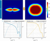
While the main direction and the degree of orientation provide valuable insight into the orientation of the scatterers, they offer only a partial view. The main scattering direction neglects the presence of other orientations that may contribute to the material's hierarchical organization; as a result, multidirectional features, which can be reconstructed in a SASTT measurement (Nielsen et al., 2024), are lost. The degree of orientation or fractional anisotropy quantifies the anisotropy of the scattering signal, where higher values indicate stronger alignment. However, this metric is based on the reconstructed scattering intensities, meaning it reflects both shape and orientation information, and it is q dependent. As illustrated in Fig. 1, the degree of orientation varies significantly between two aligned rods with different aspect ratios. The dependence on particle shape and q value makes the degree of orientation an inconsistent measure of alignment.
|
Figure 1
Simulated scattering patterns of two cylinders perfectly aligned along the vertical axis. The scattering patterns were simulated solely from their form factor contribution (Kaya, 2004 ). Cylinder 1 has an aspect ratio of 20 and cylinder 2 has an aspect ratio of 2. The integrated intensity and the degree of orientation for the cylinders vary with the q index, as shown below the scattering pattern of each cylinder. |
In this work we introduce an algorithm for extracting orientation information from SASTT experiments through the retrieval of the orientation distribution function (ODF). Unlike the degree of orientation, the ODF gives a more comprehensive view of the orientation of the scatterers, as it describes the probability of a scatterer being aligned in any given direction. Extracting orientation distributions from experimental data enables them to be used more directly as input for mechanical modeling of anisotropic materials. In fiber-reinforced composites, the mechanical response can be modeled by averaging the contribution of fibers with different orientations (Modniks & Andersons, 2013), while orientation tensors can be used to represent the orientation distribution in constitutive models (Advani & Tucker, 1987). Experimentally measured orientation information has also been used in multiscale models of hierarchical materials, such as mineralized dental tissue (Sui et al., 2015). More recently, structural information obtained from X-ray scattering tensor tomography has been directly incorporated into finite element models of fiber-reinforced composites to predict their mechanical properties (Auenhammer et al., 2024). Spatially resolved ODFs from SASTT could therefore provide experimentally measured orientation information as input for mechanical modeling.
ODFs have previously been retrieved and analyzed in several related scattering and imaging contexts. In conventional small-angle scattering, Bayesian methods have been used to infer ODFs from a limited number of measurements (Corona et al., 2021), while Rosén et al. (2018) reconstructed full 3D ODFs for axially symmetric nanofibril systems from SAXS measurements by assuming a uniform azimuthal distribution around the flow direction. SAXS-derived orientation distributions have also been widely used to characterize the alignment and dynamics of anisotropic nanoparticles in flowing and self-assembling systems (Hakansson et al., 2016; Rosén et al., 2021). In texture tomography, ODFs have been retrieved under assumptions of crystal symmetry (Carlsen et al., 2025; Frewein et al., 2025). Together, these studies demonstrate the broader relevance of orientation distribution analysis across different material systems and experimental techniques. However, conventional SAXS approaches lack the spatial resolution provided by tomography, while texture tomography methods rely on crystallographic symmetry assumptions that are not generally applicable to noncrystalline nanostructures. To date, retrieval of spatially resolved ODFs from SASTT reconstructions has not been demonstrated.
To extract the ODF, we use the deconvolution theorem of spherical harmonics. The ODF is represented as a function on the sphere using the orthonormal and complete basis set of spherical harmonics. This mathematical framework enables the separation of shape information from orientation information for SASTT reconstructions. In this study it is defined by two Euler angles, which captures the directional alignment but does not account for the rotation around an internal symmetry axis. The retrieved ODF is rotationally invariant with respect to the third Euler angle, making it suitable for samples exhibiting axial symmetry, such as rods or discs. In diffusion-weighted MRI, spherical harmonic deconvolution was used to resolve white-matter fiber orientation in the brain (Tournier et al., 2004). Additionally, a similar approach was used in crystallographic texture analysis, although only in two dimensions (Langelaan et al., 2002). In this work, we implement spherical harmonic deconvolution to retrieve the ODF from reconstructed 3D RSMs in SASTT experiments. The algorithm is applied to a plasmonic material, containing gold nanorods in a polymer matrix, to demonstrate how the quantitative ODF reveals the orientation of nanorods within the material.
2. Method
2.1. Algorithm
Scattering is typically described as the q-dependent Fourier transform of the electron density of the scatterer and can be separated into two main contributions: the form factor, which explains the shape and size of the scatterer, and the structure factor, which accounts for interparticle interactions. Additional factors, such as the number of scatterers and their electron-density contrast, also contribute to the intensity but remain independent of q (Guinier & Walker, 1955). In this study, we assume there is a q region without interparticle interactions that contributes to the scattering. As a result, the structure factor is disregarded and the scattering contribution comes from the form factor.
In addition to the form factor, the scattering model must also include the orientation information. The ODF is incorporated by aligning the form factor along a single, arbitrarily chosen axis and then rotating it using the rotation matrix R. As a result, the ODF becomes a function of R and describes the statistical distribution of scatterer orientations relative to the reference axis, which can be arbitrarily chosen.

where  is the modeled intensity,
 is the form factor, which depends on the scattering vector
 rotated by R,
 and
 is the ODF. The integral covers all rotations R in the space of proper rotations SO(3).
To model the functions f and p, spherical harmonics were used, as they provide an orthogonal basis set, allowing any square-integrable function to be expressed as an expansion of these basis functions:

 is a square-integrable function on the sphere, and it is expressed as a sum of all spherical harmonic coefficients
 multiplied by the spherical harmonics
 .
The convolution theorem of spherical harmonics is (Driscoll & Healy, 1994)

where the coefficients  are the spherical harmonic coefficients of the form factor for a scatterer that is symmetric around its internal axis, denoted
fz. Similarly,
 are the coefficients of the spherical harmonic expansion of the ODF. As shown in equation (3), only the even-order coefficients of the form factor contribute to the modeled scattering intensity, which is why this approach is best suited for particles exhibiting axial symmetry.
In principle, equation (3) provides a direct expression for the spherical harmonic coefficients for the distribution function based on a single 2D shell extracted from the 3D RSM. Due to noise in the SASTT reconstruction, it is preferable to determine the best-fit distribution function as a solution to an overdetermined optimization problem over all q values simultaneously:

where  is the optimal ODF that minimizes the difference between the model and the experimental data.
 are the coefficients of the spherical harmonic expansion of the reconstructed 3D RSM.
 are the spherical harmonic coefficients for the form factor, and are the spherical harmonic coefficients for the ODF.
The spherical harmonic coefficients, , for the experimental data are obtained through a SASTT experiment and a reconstruction of the 3D RSM, and the form factor coefficients, , are modeled. Then, the ODF coefficients,  , are obtained through minimization:

where  ,
 and
 . Standard linear algebra techniques, in this case the linear least-squares method, are used to obtain the coefficients
 .
2.2. Implementation
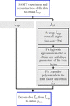
The workflow of the algorithm is illustrated in Fig. 2. A SASTT experiment followed by reconstruction of the data is used to obtain the spherical harmonic coefficients  . These coefficients serve two purposes: they are directly used in the deconvolution step, and they provide a basis for modeling the form factor coefficients .
|
Figure 2
Overview of the algorithm workflow. |
By averaging the 3D RSM over all directions, the resulting scattering intensity corresponds to that of a random orientation distribution of the scatterers. The data can be reduced to a 1D
I(q) curve, analogous to what is obtained in conventional SAXS experiments of randomly oriented scatterers. The resulting
I(q) curve is then analyzed using standard SAXS fitting tools, such as SASview (Shrestha et al., 2026) or SASfit (Breßler et al., 2015) to extract the form factor. As with all SAXS-based modeling, prior knowledge of the sample is important, since multiple models may fit the data equally well. Currently implemented shapes for form factor fitting include cylinders, capped cylinders, discs and ellipsoids, all of which exhibit axial symmetry. The algorithm also supports polydispersity, and additional shape distributions and form factors can be easily incorporated.
The model that best matches the
I(q) curve is then fitted with Legendre polynomials (a special case of spherical harmonics for functions that are symmetric around a central axis), to obtain the spherical harmonic coefficients . These are deconvolved from  to obtain .
2.3. Model system
To verify and test the algorithm, a 500 µm-thick film composed of gold nanorods embedded in a poly(methyl methacrylate) (PMMA) matrix was used. This type of system was previously used to demonstrate how upscaling of plastic plasmonic systems is possible, which has practical relevance for hydrogen sensing (Darmadi et al., 2020). This plasmonic material has previously been studied using scanning SAXS in two dimensions (Darmadi et al., 2023), but only the 3D characterization reveals how the gold nanorods are distributed and oriented within the polymer matrix. Their spatial arrangement and directionality influence the overall plasmonic behavior of the composite (Darmadi et al., 2023).
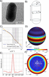
This material was selected as a model system due to the well defined shape of the scatterers, which can be modeled as capped cylinders (see Fig. 3), with the structure factor having little impact in the q range 0.014 < q < 0.042 Å−1.
|
Figure 3
(a) shows a transmission electron microscopy image of the gold nanorod. (b) shows the model of the gold nanorod that was used for the form factor modeling, which is a capped cylinder of C = r = 150 Å and L = 500 Å, with a lognormal distribution of the radii. (c) shows the radial integration of the averaged reconstruction as well as the modeled form factor, with the purple dotted line showing the q value that is depicted in (d), (e) and (f). (d) and (f) show the values of the form factor on a 3D sphere and in a pole figure, respectively. (e) shows the values of the form factor for different θ. As the form factor is axially symmetric it depends only on θ and not ϕ. |
The plastic plasmonic samples were produced using the process described by Darmadi et al. (2023), where they were synthesized in a water-based seed growth process, then mixed with the PMMA powder. The gold nanorods in the PMMA (0.05 wt% of Au) were first extruded into short filament sections of 1.75 mm in diameter, placed next to each other and pressed into plates. Cylindrical samples were milled from the plates and mounted on a needle. The sample was placed on a two-axis goniometer, aligned to the center of rotation of the goniometer, and measured for various tilts and rotations, resulting in 331 projections. The SASTT experiment is described in more detail elsewhere (Liebi et al., 2015). The SASTT experiments were performed at the cSAXS beamline of the Swiss Light Source at the Paul Scherrer Institute in Switzerland. The energy of the beam was 11.2 keV with a beam size of 7.5 µm (vertical) × 28 µm (horizontal), with continuous scanning in y and step size  µm2. The sample-to-detector distance was 7 m and the exposure time was 0.05 s. The reconstructions were performed with MUMOTT 2.1 (Nielsen et al., 2025), using Gaussian kernels with a grid scale of 6 and no regularization, and then recalculated to spherical harmonic coefficients with
 .
3. Results and discussion
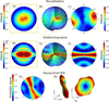
To demonstrate the ODF extracted by the algorithm, a representative voxel from the middle of the sample was used, as shown in Fig. 4.
|
Figure 4
3D RSM of the reconstruction. The modeled form factor is shown in (d)–(f) and the ODF is presented in (g)–(h). (b) and (e) illustrate the 3D RSM using concentric spheres at q values around q = 0.038 Å−1, the same q value that is marked in Fig. 3 . (a) and (d) show planar cuts through the 3D RSM, which correspond to the scattering pattern that would be observed if the voxel was measured in isolation, with the incident X-rays perpendicular to the plane of the cut. (c), (f) and (g) show pole figures evaluated at q = 0.038 Å−1. The ODF is visualized in (h) as a 3D representation where both the radial distance from the center and color indicate the probability of finding the gold nanorods aligned along that direction, and it shows two alternative viewing angles of the same ODF. |
For the plastic plasmonic sample, the reconstructed 3D RSM exhibits two poles in the pole figure [Fig. 4(c)], in contrast to the ring-like scattering pattern observed in the modeled form factor [Fig. 4(f)]. The reconstruction of the plastic plasmonic sample was used to find an average q-dependent intensity, over all angles,
I(q) [see Fig. 3(c)], which was used to fit the parameters of the form factor. The ODF was obtained by deconvolving the form factor from the reconstructed data, as described in equation (4). The ODF for the representative voxel in the middle of the sample displays a ring-like probability distribution [Figs. 4(g) and 4(h)], indicating that the gold nanorods are predominantly oriented within a plane, with no strong preferential direction within that plane. The main scattering direction of the reconstruction corresponds to the normal vector of this orientation plane. This planar alignment is likely a result of the sample preparation process, during which the material was first extruded and then pressed into thin plates. The sequence of processing steps probably induced the observed in-plane alignment of the nanorods. These findings demonstrate that the deconvolution algorithm yields a quantitative ODF, capturing the full directional distribution of the nanorods. More generally, such distribution-based information may be valuable for heterogeneous anisotropic materials in which broad, planar or multiple orientations coexist, including fibrous biological materials (Liao et al., 2005) and flow- or processing-aligned particle systems (Rosén et al., 2021; Wells et al., 2015). In these cases, a full ODF can reveal orientational features that are not captured by a single main direction or scalar measure of anisotropy.
Notably, the ODF shown in Fig. 4(g) includes negative values in the pole figure. These negative regions are not visible in the 3D representation of the ODF in Fig. 4(h). Negative probabilities are nonphysical and arise as artifacts from using spherical harmonics as the basis set, which does not inherently have a positivity constraint. As a result, the coefficients obtained through deconvolution may yield negative values when evaluated on the sphere. For future developments, regularization that penalizes negative values can be incorporated into the deconvolution algorithm, similarly to what has been done in diffusion-weighted MRI (Tournier et al., 2007). This would help enforce a strictly positive probability distribution, at the cost of increased computational complexity. Alternatively, the ODF can be transformed to a basis set in which positivity can be imposed more directly, for example through non-negative coefficients. A transformation between orthogonal basis sets can be implemented as a linear transformation and would therefore require only an additional matrix multiplication. Such an approach could provide a computationally simple way of incorporating a positivity constraint into the current framework.
When using the deconvolution algorithm, several limitations must be considered. One key limitation concerns the influence of the structure factor on the scattering signal. The algorithm does not account for how interparticle interactions impact the 3D RSM, but relies solely on the form factor. Many form factors can be easily modeled in three dimensions; however, the structure factor's angular and q dependency,  , is unknown and therefore not included in the model. Since the deconvolution is performed across a range of q values, it is essential that a region exists where the scattering is dominated by the form factor alone. In practice, this means that there is an interval of the radially integrated intensity curve
I(q) that can be accurately fitted using the form factor only. For the plastic plasmonic sample, only the q values near q = 0.038 Å−1 were used, as shown in Fig. 3.
Another important consideration when using the algorithm is the number of spherical harmonic basis functions applied in both form factor fitting and reconstruction, which must share the same maximum degree,
lmax. Using a higher
lmax for one of the properties, for example the form factor, would imply extracting more information from the ODF than is present in the reconstructed data, which is not physically meaningful. Using too few spherical harmonics may lead to sharp features not being properly resolved. On the other hand, increasing
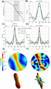
lmax leads to overfitting of noise in the reconstruction. This effect is illustrated in Fig. 5, where higher
lmax values result in fitting noise rather than meaningful structural features.
|
Figure 5
(a) shows the I(q) of the form factor; the gray area marks the interval that is used to find the ODF. The three marked q values are the same q values that are used to show  in (b)–(d). The ODFs are shown as pole figures and in 3D representations for  and  , in (e) and (f), respectively. |
A comparison between the analytically calculated form factor [Fig. 3(d)] and the fitted form factor used in the reconstruction [Figs. 4(d)–4(f)] reveals that the analytical form factor exhibits less oscillation between high- and low-intensity values. Hence, when fitting the form factor with too few Legendre functions, and indirectly
lmax, the form factor will oscillate more over the sphere. This is furthermore evident in Figs. 5(b)–5(d), where the form factor fit oscillates more than the actual form factor values. At low q values, both expansion orders adequately capture the main peak of the form factor. However, as q increases, the quality of the fit deteriorates. The higher-order expansion () better captures the width of the main peak but introduces oscillations outside the peak region. In contrast, the lower-order expansion () fails to fit the peak width but results in a smoother overall fit. This trade-off is reflected in the resulting ODFs. For , the ODF appears smoother and exhibits a ring-like distribution. The low
lmax does not fit the width of the form factor peak well. Since the form factor and ODF are convolution inverses, a broader form factor yields a narrower ODF to maintain consistency with the reconstruction. On the other hand, using a high
lmax can lead to the inclusion of noise in the reconstruction, which propagates into the ODF as artificial oscillations. While the width of the ODF may be more accurately captured in this case, distinguishing true structural features from noise-induced artifacts becomes more challenging. To perform a reliable deconvolution, it is therefore optimal to use the highest possible
lmax that does not overfit the noise in the reconstruction – in this project was used. This balance ensures the most accurate and physically meaningful estimation of the ODF.
As outlined in equation (3), the algorithm assumes that the form factor is axially symmetric, meaning it is invariant under rotation around an internal axis, since only the  order spherical harmonic coefficients of the form factor are used. Due to this symmetry constraint, the algorithm does not recover the full ODF, but rather only the directional orientation, while the rotation around the scatterers' internal axis remains undetermined. Extending the method to retrieving the three Euler angles is therefore not feasible within the current framework. Consequently, the method is best suited for scatterers with simple, symmetric geometries such as cylinders, discs or ellipsoids.
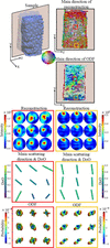
The deconvolution algorithm was used on the entire sample to obtain an ODF in each voxel of the sample (see Fig. 6).
|
Figure 6
The top-left figure illustrates the sample, with a semi-transparent plane indicating a cross-sectional cut. This cut is shown in two dimensions, and the main directions of both the reconstruction and the ODF are color-coded according to the color wheel. Directions perpendicular to the cut appear in grayer tones. Pole figures from the reconstruction are shown for two distinct regions of the sample, one from the center and one from the edge. The main direction of the scattering and the degree of orientation (denoted DoO) are represented by color-coded bars. The direction of each bar corresponds to the main orientation projected onto the yz plane, while its color and length are scaled according to the degree of orientation. The ODF is visualized in its 3D representation. |
To illustrate differences in scatterer orientation across the sample, two sub-regions were analyzed. As shown in Fig. 6, a region near the center of the sample exhibits orientations that point along the x axis. This is reflected in the reconstruction, with poles along the same direction. However, visualization of the main direction in two dimensions is limited when the main direction is along the x axis, as it only shows the projection of the eigenvector onto the viewing plane and does not take into account out-of-plane components. The corresponding ODF in this central region reveals a broad distribution of orientations, occasionally displaying multidirectional features, and with colors and lengths indicating a lower degree of alignment. In contrast, a region closer to the edge of the sample shows that nanorods are oriented primarily along the y axis, which is also captured in the main direction bars. The ODF in this region is narrower and points predominantly along the z axis, suggesting a higher degree of alignment. These observations imply that the central region of the sample is less ordered, while the edges exhibit greater alignment. This variation may result from the processing sequence. Alignment comes from the filament extrusion where the material is pushed through a small die and forced into filaments, which were in turn placed next to each other in the extrusion direction. In the subsequent step, when the parallel filaments were pressed into plates, alignment was more strongly induced near the pressing surface.
Fig. 6 highlights a key distinction between the most probable orientation of the scatterers, as revealed by the ODF, and the main scattering direction obtained from the reconstruction. In the case of the plasmonic plastic film, the main scattering direction is perpendicular to the ring-like distribution of gold nanorods. In scattering experiments the main direction of scattering does not necessarily correspond to the most probable orientation of the scatterers; it can also lie perpendicular to the main scattering direction. In three dimensions, however, the term perpendicular encompasses an entire ring of directions, and without the ODF it is not possible to determine whether all these directions are equally probable or if certain orientations are preferred. The ODF provides this critical information, revealing not only the dominant orientation but also the spread and shape of the distribution. Moreover, the ODF can uncover multidirectional features that are not apparent when relying solely on the eigenvectors used to define the main direction. While the degree of orientation derived from the reconstruction offers a scalar measure of the alignment, the ODF gives a more detailed picture, showing how sharply the orientation of scatterers is distributed and which directions are probable beyond the main one.
In summary, the deconvolution yields a quantitative ODF, providing insights that go beyond the main scattering direction and degree of orientation. Unlike the degree of orientation, which is influenced by both the form factor and the orientation information, the ODF isolates directional information, enabling a more nuanced analysis of structural orientation. Its quantitative interpretation, however, relies on an accurate form factor model, an appropriate q range, sufficient angular representation and a reliable SASTT reconstruction, as modeling errors may otherwise be absorbed into the ODF as apparent orientational information. When these conditions are fulfilled, the ODF provides a physically meaningful description of the particle orientation distribution. This is particularly valuable in systems with multiple or complex orientation distributions, where a quantitative ODF is essential for accurate material characterization.
4. Conclusions
The algorithm presented in this work expands the current toolbox for SASTT experiments by enabling the retrieval of a quantitative ODF. Using the convolution theorem of spherical harmonics as the mathematical framework, the directional information is decoupled from the shape and size information, referred to as the form factor. The form factor is modeled by assuming that the scatterers are randomly oriented and averaging all directions to obtain I(q). Legendre polynomials are fitted to the curve to obtain the spherical harmonic expansion coefficients of the form factor. The form factor information is then deconvolved from the reconstruction to obtain the ODF.
This approach allows for the extraction of a voxel-wise quantitative ODF, providing the probability of alignment in any direction, rather than just identifying the most probable orientation. Notably, when the form factor is accounted for, the orientation of the scatterers may differ significantly from the main scattering direction. The algorithm is applicable to samples containing scatterers that can be approximated as simple, axially symmetric shapes, and within a q range where the scattering is dominated by the form factor, with a negligible contribution from the structure factor. A known limitation of the spherical harmonic representation is the lack of a positivity constraint, which can result in nonphysical negative values in the ODF. Future work may address this by incorporating regularization or positivity-enforcing constraints to suppress those artifacts.
Overall, this development opens new possibilities for detailed orientation analysis in anisotropic materials using SASTT, offering a more complete and quantitative understanding of the internal structural organization.
Acknowledgements
We gratefully acknowledge the Paul Scherrer Institute for providing beamtime at the cSAXS beamline of the Swiss Light Source (SLS) under proposal 20201560. We also thank the cSAXS beamline staff for their support during the experiment, with special thanks to Ana Diaz for assistance in setting up the measurements. Additional thanks go to Adrian Rodriguez-Palomo for help with sample preparation, Jonathan Avaro for support during the experiments, and Leonard Nielsen for assistance with data analysis and MUMOTT reconstructions. This work was performed with assistance from Microsoft 365 Copilot for language clarity and proofreading. The final content, interpretations and conclusions presented in this article are entirely the authors'. The views expressed are those of the authors and do not necessarily reflect those of the European Union or the European Research Council Executive Agency; neither the EU nor the granting authority can be held responsible for them. Open access publishing facilitated by ETH-Bereich Forschungsanstalten, as part of the Wiley–ETH-Bereich Forschungsanstalten agreement via the Consortium of Swiss Academic Libraries.
Conflict of interest
The authors declare no conflict of interest.
Data availability
The software and data required to reproduce the results presented in this work are available in the associated Zenodo repository at https://doi.org/10.5281/zenodo.22281182. The source code is also available from the corresponding GitLab repository.
Funding information
This work was supported by the European Research Council Starting Grant MUMOTT (ERC-2020-StG 949301), funded by the European Union. MC and CA acknowledge funding from the European Union's Horizon 2020 research and innovation program under the Marie Skłodowska-Curie grant agreement No. 884104. IÖ, SL, CM and KMP acknowledge financial support from the Swedish Foundation for Strategic Research project RMA15-0052.
References
 Advani, S. G. & Tucker, C. L. (1987). J. Rheol. 31, 751–784.
CrossRef
CAS
Google Scholar
Auenhammer, R. M., Kim, J., Oddy, C., Mikkelsen, L. P., Marone, F., Stampanoni, M. & Asp, L. E. (2024). npj Comput Mater, 10, 50.
CrossRef
Google Scholar
Basser, P. J. & Pierpaoli, C. (1996). J. Magn. Reson. B. 111, 209–219.
CrossRef
CAS
PubMed
Google Scholar
Breßler, I., Kohlbrecher, J. & Thünemann, A. F. (2015). J. Appl. Cryst. 48, 1587–1598.
Web of Science
CrossRef
IUCr Journals
Google Scholar
Bunk, O., Bech, M., Jensen, T. H., Feidenhans'l, R., Binderup, T., Menzel, A. & Pfeiffer, F. (2009). New J. Phys. 11, 123016.
Web of Science
CrossRef
Google Scholar
Carlsen, M., Malamud, F., Modregger, P., Wildeis, A., Hartmann, M., Brandt, R., Menzel, A. & Liebi, M. (2025). J. Appl. Cryst. 58, 484–494.
Web of Science
CrossRef
CAS
IUCr Journals
Google Scholar
Corona, P. T., Silmore, K. S., Adkins, R., Lang, C., Lettinga, M. P., Swan, J. W., Leal, L. G. & Helgeson, M. E. (2021). Phys. Rev. Mater. 5, 065601.
Web of Science
CrossRef
Google Scholar
Darmadi, I., Östergren, I., Lerch, S., Lund, A., Moth-Poulsen, K., Müller, C. & Langhammer, C. (2023). Acc. Chem. Res. 56, 1850–1861.
CrossRef
CAS
PubMed
Google Scholar
Darmadi, I., Stolaś, A., Östergren, I., Berke, B., Nugroho, F. A. A., Minelli, M., Lerch, S., Tanyeli, I., Lund, A., Andersson, O., Zhdanov, V. P., Liebi, M., Moth-Poulsen, K., Müller, C. & Langhammer, C. (2020). ACS Appl. Nano Mater. 3, 8438–8445.
CrossRef
CAS
Google Scholar
Driscoll, J. R. & Healy, D. M. (1994). Adv. Appl. Math. 15, 202–250.
CrossRef
Web of Science
Google Scholar
Frewein, M. P. K., Mason, J., Maier, B., Cölfen, H., Medjahed, A., Burghammer, M., Allain, M. & Grünewald, T. A. (2024). IUCrJ 11, 809–820.
CrossRef
CAS
PubMed
IUCr Journals
Google Scholar
Gao, Z., Guizar-Sicairos, M., Lutz-Bueno, V., Schröter, A., Liebi, M., Rudin, M. & Georgiadis, M. (2019). Acta Cryst. A75, 223–238.
Web of Science
CrossRef
IUCr Journals
Google Scholar
Georgiadis, M., Guizar-Sicairos, M., Zwahlen, A., Trüssel, A. J., Bunk, O., Müller, R. & Schneider, P. (2015). Bone 71, 42–52.
CrossRef
CAS
PubMed
Google Scholar
Grünewald, T. A., Johannes, A., Wittig, N. K., Palle, J., Rack, A., Burghammer, M. & Birkedal, H. (2023). IUCrJ 10, 189–198.
Web of Science
CrossRef
PubMed
IUCr Journals
Google Scholar
Guinier, A. & Walker, C. B. (1955). Small-Angle Scattering of X-rays. New York: John Wiley Sons.
Google Scholar
Håkansson, K. M., Lundell, F., Prahl-Wittberg, L. & Söderberg, L. D. (2016). J. Phys. Chem. B 120, 6674–6686.
PubMed
Google Scholar
Kaya, H. (2004). J. Appl. Cryst. 37, 223–230.
Web of Science
CrossRef
CAS
IUCr Journals
Google Scholar
Langelaan, G., Delannay, L., Verpoest, I. & Van Houtte, P. (2002). J. Appl. Cryst. 35, 327–337.
Web of Science
CrossRef
CAS
IUCr Journals
Google Scholar
Liao, J., Yang, L., Grashow, J. & Sacks, M. S. (2005). Acta Biomaterialia 1, 45–54.
CrossRef
PubMed
Google Scholar
Liebi, M., Georgiadis, M., Kohlbrecher, J., Holler, M., Raabe, J., Usov, I., Menzel, A., Schneider, P., Bunk, O. & Guizar-Sicairos, M. (2018). Acta Cryst. A74, 12–24.
CrossRef
IUCr Journals
Google Scholar
Liebi, M., Georgiadis, M., Menzel, A., Schneider, P., Kohlbrecher, J., Bunk, O. & Guizar-Sicairos, M. (2015). Nature 527, 349–352.
Web of Science
CrossRef
CAS
PubMed
Google Scholar
Liebi, M., Lutz-Bueno, V., Guizar-Sicairos, M., Schönbauer, B. M., Eichler, J., Martinelli, E., Löffler, J. F., Weinberg, A., Lichtenegger, H. & Grünewald, T. A. (2021). Acta Biomaterialia 134, 804–817.
CrossRef
CAS
PubMed
Google Scholar
Modniks, J. & Andersons, J. (2013). Composites Part B 54, 188–193.
CrossRef
CAS
Google Scholar
Nielsen, L. C., Carlsen, M., Wang, S., Baroni, A., Tänzer, T., Liebi, M. & Erhart, P. (2025). J. Appl. Cryst. 58, 1834–1845.
Web of Science
CrossRef
CAS
IUCr Journals
Google Scholar
Nielsen, L. C., Erhart, P., Guizar-Sicairos, M. & Liebi, M. (2023). Acta Cryst. A79, 515–526.
Web of Science
CrossRef
IUCr Journals
Google Scholar
Nielsen, L. C., Tänzer, T., Rodriguez-Fernandez, I., Erhart, P. & Liebi, M. (2024). J. Synchrotron Rad. 31, 1327–1339.
Web of Science
CrossRef
CAS
IUCr Journals
Google Scholar
Pabisch, S., Wagermaier, W., Zander, T., Li, C. & Fratzl, P. (2013). Methods Enzymol. 532, 391–413.
Web of Science
CrossRef
CAS
PubMed
Google Scholar
Rodriguez-Fernandez, I., Bretschneider, T., Menzel, A., Suljevic, O., Sommer, N. G., Weinberg, A., Appel, C., Liebi, M., Diaz, A., Pircher, L., Hellmich, C., Schwarze, U. Y., Lichtenegger, H. C. & Grünewald, T. A. (2025). Acta Biomater. 193, 623–631.
CAS
PubMed
Google Scholar
Rodriguez–Palomo, A., Østergaard, M. & Birkedal, H. (2024). Adv. Funct. Mater. 34, 2307026.
Google Scholar
Rosén, T., Brouzet, C., Roth, S. V., Lundell, F. & Söderberg, L. D. (2018). J. Phys. Chem. C 122, 6889–6899.
Google Scholar
Rosén, T., Hsiao, B. S. & Söderberg, L. D. (2021). Adv. Mater. 33, 2001238.
PubMed
Google Scholar
Shrestha, S. et al. (2026). SasView, Version 6.2.0, https://doi.org/10.5281/zenodo.20270235.
Google Scholar
Schaff, F., Bech, M., Zaslansky, P., Jud, C., Liebi, M., Guizar-Sicairos, M. & Pfeiffer, F. (2015). Nature 527, 353–356.
Web of Science
CrossRef
CAS
PubMed
Google Scholar
Sui, T., Ying, S. Q., Baimpas, N., Landini, G. & Korsunsky, A. M. (2015). Appl. Mech. Mater. 798, 339–343.
CrossRef
Google Scholar
Tournier, J. D., Calamante, F. & Connelly, A. (2007). NeuroImage 35, 1459–1472.
CrossRef
PubMed
Google Scholar
Tournier, J. D., Calamante, F., Gadian, D. G. & Connelly, A. (2004). NeuroImage 23, 1176–1185.
CrossRef
PubMed
Google Scholar
Wells, H. C., Sizeland, K. H., Kirby, N., Hawley, A., Mudie, S. & Haverkamp, R. G. (2015). ACS Biomater. Sci. Eng. 1, 1026–1038.
CrossRef
CAS
PubMed
Google Scholar
This is an open-access article distributed under the terms of the Creative Commons Attribution (CC-BY) Licence, which permits unrestricted use, distribution, and reproduction in any medium, provided the original authors and source are cited.
| JOURNAL OF APPLIED CRYSTALLOGRAPHY |