

 menu


computer programs
 | JOURNAL OF APPLIED CRYSTALLOGRAPHY |
 access
SAS_MoCa: software for small-angle scattering data analysis of large unilamellar vesicles

aUniversity of Graz, Institute of Molecular Biosciences, NAWI Graz, 8010 Graz, Austria, bField of Excellence BioHealth – University of Graz, Graz, Austria, and cBioTechMed Graz, 8010 Graz, Austria
*Correspondence e-mail: [email protected]
Small-angle X-ray or neutron scattering (SAXS/SANS) analysis of large unilamellar vesicles (LUVs) is often limited by high-dimensional bilayer models and the lack of dedicated, statistically rigorous workflows. Here, we introduce SAS_MoCa, an open-source Python package that integrates a compositional scattering density profile (SDP) description of lipid bilayers with a separated form factor (SFF) treatment of vesicle size and polydispersity, and couples these highly parameterized models to an adaptive thermodynamic simulated annealing algorithm formulated within a constrained Bayesian framework. SAS_MoCa enables users to incorporate quantitative prior information from, e.g., previous SAXS/SANS studies, dynamic light scattering, NMR or molecular simulations, and returns full posterior parameter distributions, uncertainties (reported as medians and median absolute deviations) and correlations even from single SAXS curves. Validation on SAXS-only data of LUVs of varying compositions demonstrates that the method yields reproducible structural parameters with uncertainties comparable to those from joint SAXS/contrast-variation SANS analyses. The modular architecture of SAS_MoCa facilitates extension to additional lipid systems and future joint SAXS/SANS or SANS-only applications.
Keywords: small-angle X-ray scattering; large unilamellar vesicles; Bayesian inference; membrane structure; open-source software.
1. Introduction
Lipid vesicles of defined size and composition are highly popular platforms in fundamental life science/soft matter research and numerous biotech applications (Pabst et al., 2014 ). In particular organelle-sized vesicles, known as large unilamellar vesicles (LUVs) with sizes of around 100 nm, often serve as minimal models of cellular membranes, extracellular vesicles or lipid nanoparticles for diverse drug-delivery formulations [see e.g. Chacko et al. (2020)]. Small-angle scattering (SAS) stands as one of the most powerful and non-invasive techniques for probing LUV structure at mesoscopic length scales (Semeraro et al., 2024). However, extracting meaningful structural parameters from SAS data typically demands significant expertise in scattering theory, model selection and statistical validation.
Currently, popular SAS analysis tools such as SasView (Krzywon et al., 2025) lack a bespoke workflow tailored specifically to LUVs, while a previously dedicated online tool, Vesicle Viewer (Lewis-Laurent et al., 2021), is no longer maintained. Alternatively, the scattering length density profile of lipid bilayers can be analyzed via a heuristic combination of Gaussian curves with the routine LIPMIX, embedded in the ATSAS software (Konarev et al., 2021), extending a previously reported full-q-range analysis of multilamellar and unilamellar vesicles (Pabst et al., 2000; Pabst et al., 2003). However, none of these tools combine compositional information of the lipid bilayer with a vesicle size and polydispersity analysis. Consequently, high fidelity scattering data analysis of LUVs presents a pressing bottleneck and significant barrier for progress in fundamental biological membrane research and biotechnological applications of these systems.
To address these challenges, we present SAS_MoCa, an open-source tool enabling Bayesian-constrained compositional analysis of LUV small-angle X-ray scattering (SAXS) data (Semeraro & Pabst, 2026). Specifically, SAS_MoCa provides a multiscale analysis that integrates the scattering density profile (SDP) model for high-resolution bilayer structure (Kučerka et al., 2008) and the separated form factor (SFF) model for vesicle size and size polydispersity (Pencer et al., 2006). The package provides a unified, open-source framework that streamlines data import, curve fitting, result aggregation and visualization, thereby lowering the barrier to entry for non-specialists in scattering analysis.
At the core of the package is an adaptive stochastic minimization engine tailored to explore the high-dimensional parameter space characteristic of SDP modeling of LUVs. This engine is formulated within a Bayesian framework, allowing users to incorporate prior information—such as bilayer thickness or vesicle radius—and to obtain full posterior distributions for all adjustable parameters. While deterministic optimizers (e.g. Levenberg–Marquardt) offer rapid convergence to local minima, they lack the capacity to quantify parameter uncertainties or explore complex likelihood landscapes. SAS_MoCa bridges this gap by implementing constrained Bayesian inference that provides full statistical characterization—median values, credible intervals and parameter correlations—in a matter of minutes even on a standard laptop.
SAS_MoCa thus offers a unified framework for integrating SAXS measurements with diverse quantitative priors. Instead of relying exclusively on the scattering curve, users can combine it with (i) literature values from previous joint SAXS/SANS studies of analogous lipid systems, (ii) independent experimental measurements such as, e.g., dynamic light scattering (DLS) for vesicle size and (iii) computational results, providing high-resolution structural information beyond the intrinsic resolution of SAS. This enables knowledge transfer from well-characterized systems to new experiments and establishes a general, rigorous route for incorporating external constraints into scattering-based structural analysis.
Finally, the software architecture is deliberately modular, making it straightforward to extend the package to alternative scattering models and to tackle small-angle neutron scattering (SANS) data, including contrast-variation and joint SAXS/SANS analyses.
This manuscript is organized as follows. First, we present the scattering models and the Bayesian-stochastic fitting engine implemented in SAS_MoCa. We then validate the methodology using experimentally measured scattering data from LUVs of varying compositions and assess its performance and limitations. Finally, we summarize the main conclusions and outline avenues for future developments and extensions.
2. Program overview
2.1. Scattering form factor
The SAS_MoCa repository currently includes scattering form factors designed to analyze the bilayer structure and size of LUVs. We assume that the vesicles are fully hydrated within the lamellar fluid phase,  , and freely float in pure water. The scattering intensity of a suspension of LUVs is expressed as

where  is the number density of LUVs;
 represents the SFF contribution of the spherical LUV frame of radius
 , including polydispersity effects (Pencer et al., 2006); and the scattering amplitude
 describes the one-dimensional lipid bilayer contribution according to the SDP formalism (Kučerka et al., 2008; Frewein et al., 2021). The averaging operator
 denotes integration over a normal distribution of hydrocarbon layer thicknesses (Frewein et al., 2021). Detailed derivations of the model implementation are provided in Appendix A.
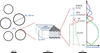
While the SFF model considers LUVs as rigid spherical frames with a given size distribution, the SDP approach treats each lipid as a collection of quasi-molecular groups (see Fig. 1), with each group contributing individually to the scattering signal (Kučerka et al., 2008). As the SDP is a compositional model, the specifics of  depend directly on lipid composition (see Fig. 1 and Appendix A). SAS_MoCa currently implements the compositional design for the following lipid systems: POPC (1-palmitoyl-2-oleoyl-sn-glycero-3-phosphocholine), DMPC (1,2-dimyristoyl-sn-glycero-3-phosphocholine) and POPE (1-palmitoyl-2-oleoyl-sn-glycero-3-phosphoethanolamine).
|
Figure 1
Schematic representation of the multiscale SFF-SDP model, from LUVs' size to the parsing of quasi-molecular groups in, e.g., POPC lipids (Kučerka et al., 2011 ). |
2.1.1. Numerical Implementation
Equation (1) defines the theoretical scattering intensity. SAS_MoCa implements this calculation within the LUV_POPC class (and analogous classes for DMPC and POPE) through a sequential modular workflow of component definitions. For users navigating the source code (e.g. sasmoca/models/LUV_POPC.py), the implementation logic follows these key steps:
(1) Initialization. The constructor parses input parameters, y, computes lipid-specific volumes (e.g.  ,
 ) and loads the scattering lengths, b, pertinent to the quasi-molecular groups of the specific compositional design from sasmoca/models/constants.py (see Table S1). Volumes and b values are combined in scattering length density,
 , values as functions of temperature and composition. The initialization further establishes the LUV geometric framework, including vesicle polydispersity and hydrocarbon layer thickness distributions.
(2) Amplitude calculation. The core membrane scattering amplitude is assembled by summing contributions from quasi-molecular groups. The code distinguishes between smooth rectangular profiles (acyl chains, hydration layers) computed via error-function Fourier transforms (FTreal_erf) and Gaussian profiles (head groups, terminal methyls) using FTreal_gauss (see Appendix A). An integration grid over the hydrocarbon thickness distribution is generated to account for thickness fluctuations  .
(3) Intensity aggregation. The scattered intensity is computed according to equation (1). The method intensity() then returns the total model curve  , where
 is a normalization scaling factor. Notably, the background term
 incorporates a sigmoidal transition at high q values. This functional form accounts for the typical unidentified scattering contributions at high q values without obscuring the structural signal in the mid-q range where the form factor oscillations reside (Semeraro et al., 2024). Current settings are optimized for
 Å,
 Å and
 .
Note that the lipid volume, , and scattering length density of suspension water,  , are automatically calculated for the sample temperature, T, by interpolating reported data. For the PC, PE and PG species considered here, lipid volumes are obtained by linear interpolation in the range 20–60 °C using the data reported by Kučerka et al. (2011), Kučerka et al. (2015) and Pan et al. (2012), respectively. The scattering length density of the suspending water is instead calculated through the water molecule volume, which in turn is obtained via a polynomial interpolation in the range 1–100 °C using standard tables [see, e.g., Harvey (1998)]. Linear coefficients for lipid volumes and polynomial coefficients for water volumes are listed in sasmoca/models/constants.py.
2.2. Minimization algorithm
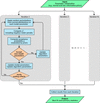
To optimize the large number of adjustable parameters of SDP-based LUV models, we employ a Monte Carlo approach that combines efficient  minimization with rapid convergence. The core of our algorithm consists of a series of thermodynamic simulated annealing (TSA) minimization runs, adapted from the work of de Vicente et al. (2003). Each iteration is independent, allowing for parallel execution. The workflow of the program is depicted in Fig. 2.
|
Figure 2
Flowchart of the SAS_MoCa minimization algorithm. The process begins with parameter initialization, proceeds through iterative TSA loops involving perturbations and acceptance checks, and concludes with the collection of best-fit parameters and statistical analysis. |
2.2.1. Initialization
In SAS_MoCa, we initialize each adjustable parameter, y, on the basis of an initial guess and prior knowledge. Users can define two types of priors:
(a) Non-informative priors, i.e. hard boundaries. Users can set minimum ( ) and maximum (
 ) limits. This corresponds to a rectangular prior distribution, referred to as a non-informative prior, where all values within the range are equally probable.
(b) Informative priors. Users can specify a normally distributed prior,  , by setting its mean,
 , and relative standard deviation,
 . By default we impose additional hard boundaries at
 around for computational stability.
Beyond model parameters, users can configure global options, such as the total number of TSA iterations,  . These iterations can be executed sequentially or distributed across multiple parallel processes.
2.2.2. Single TSA iteration
Each TSA iteration begins by calculating the initial reduced  from the starting parameter set. The algorithm then enters an iterative loop wherein adjustable parameters are perturbed, an acceptance probability is computed and the new parameter set is evaluated. This loop continues until specific termination criteria are met.
2.2.2.1. Apply random perturbations
In each step, the current model parameters are modified by small random perturbations. Specifically, every adjustable parameter
yi is shifted by a value drawn from a normal distribution centered at zero, with a standard deviation equal to  , where β is a tunable scale factor that adapts dynamically throughout the minimization.
2.2.2.2. Negative water penalty
We incorporate a penalty term into the reduced calculation to suppress configurations that yield non-physical water volume fractions within the lipid bilayer. In the SDP formalism, the head-group hydration layer volume is obtained by subtracting the volumes of the quasi-molecular lipid groups located in the head-group region from the total hydration shell volume. If the fitted parameters imply a lipid head-group volume larger than the available shell volume, the residual water volume becomes negative and thus unphysical. To detect and penalize such cases systematically, we implement the following procedure.
First, the negative_water() method discretizes the bilayer profile and counts the number of grid points,  , where the local water volume fraction falls below a threshold of −0.01. This count is then converted into a multiplicative penalty factor that is applied to the reduced prior to the acceptance step. The effective
 is defined as

where λ is a user-defined scaling factor (default neg_water_scale: 5, set in the YAML configuration file settings.yml). Because the acceptance probability depends exponentially on  [equation (3)], even moderate values of λ strongly disfavor parameter sets with non-physical water distributions, guiding the TSA algorithm away from such regions without introducing hard constraints that could trap the optimization.
2.2.2.3. Compute probability of acceptance
We evaluate each trial set of model parameters on the basis of the effective reduced and the distances from the prior centers. For the kth iteration within a TSA loop, the acceptance probability
pk is given by

where  is the annealing temperature parameter and
 represents the normal prior for the ith adjustable model parameter. The first factor corresponds to the standard thermodynamic simulated annealing criterion (de Vicente et al., 2003), while the product over i implements the prior-based acceptance modification described by Frewein et al. (2019).
2.2.2.4. Evaluate new set of parameters
We accept or reject the proposed set of randomly perturbed parameters by comparing a random value  against
pk:
(a) If  , the kth set is accepted. It replaces the previous parameter set and is stored as the best set of parameters. Furthermore, if
 (the lowest found so far), we update
 .
(b) If  and
 , the kth set is accepted and replaces the previous one. However, the best parameters and remain unchanged.
(c) If and  , the kth set is rejected, and the previous set remains unchanged.
We also use this assessment to update algorithm parameters. Specifically, we compute the acceptance/rejection rates to adjust the TSA temperature (de Vicente et al., 2003), and we dynamically modify the scale factor β to maintain an acceptance rate between 60% and 70%.
2.2.2.5. Check for ending criteria
The TSA loop terminates when a user-defined maximum number of repetitions is reached (default maxcount: 100000, configured in settings.yml) or convergence is detected. Convergence is determined by monitoring the cumulative likelihood of approaching a user-defined target  . Specifically, we check if

where the threshold (default conv_threshold: 4) can be configured in settings.yml. Note that if  , we automatically update to the new minimum, ensuring the convergence criterion adapts to the best solution found.
2.2.3. Collecting best results and summary statistics
Finally, we collect the final, best set of parameters and from each independent TSA run to compute summary statistics. This collection yields a posterior-like distribution for each model parameter, from which we calculate median values, the median absolute deviation (MAD) from medians and the Pearson correlation coefficients.
2.3. Statistical background: Bayesian inference and information update
The core philosophy of SAS_MoCa rests on the Bayesian principle of updating beliefs. In traditional least-squares fitting, the goal is often to find a single set of parameters that minimizes the discrepancy between model and data, implicitly assuming that the data contain sufficient information to determine every parameter uniquely. However, in complex scattering models such as the SDP model, the scattering signal often lacks the resolution to constrain all physical parameters simultaneously.
Bayesian inference addresses this limitation by treating parameters as stochastic variables characterized by probability distributions. The analysis exploits Bayes' theorem:

where  is the posterior distribution of the parameters
yi given the data,
 is the likelihood (how well the model fits the data) and
 is the prior distribution representing our knowledge before `seeing' the data (Ramachandran & Tsokos, 2015).
In the context of SAS_MoCa, the stochastic minimization algorithm samples this posterior distribution. The result of this sampling process reveals the extent to which the experimental data have updated our initial assumptions. We can distinguish two limiting behaviors depending on the degree of this update:
(1) Data-dominated updates (`sensitive' parameters). When the experimental signal is strong and informative regarding a specific parameter
yi, the likelihood term is a narrow and bell-shaped distribution. The posterior distribution is dominated by the data, regardless of the shape of the prior. Even if we shift the prior mean significantly, the resulting posterior remains stable and centered near the value dictated by the scattering curve. In this regime, the data have successfully `updated' the prior, extracting new information that was not present in our initial guess.
(2) Prior-dominated updates (`non-sensitive' parameters). Conversely, when the data contain insufficient information to constrain a parameter (e.g. due to limited q range, low contrast or high noise), the likelihood distribution is rather featureless over a wide range of possible parameter values. In such cases, the posterior distribution closely mirrors the prior distribution, that is  . The Bayesian update fails to shift the distribution because the analysis cannot discriminate between different values. Here, the final result is essentially a confirmation of our prior assumption, not a discovery derived from the experiment.
This framework changes the interpretation of the output. The primary goal of SAS_MoCa is not merely to provide point estimates such as medians and deviations but to visualize the shift between prior and posterior. By inspecting the posterior histograms alongside the priors (as demonstrated in Section 4), users can immediately assess whether a parameter was truly determined by the experiment or constrained by external knowledge. If the posterior overlaps significantly with the prior, either the data confirm the previous belief or the user must acknowledge that the result relies on the validity of that prior. If the posterior is distinct from the prior, the experiment has provided independent structural insight. This distinction empowers a more rigorous workflow: users are encouraged to test the robustness of their results by varying the priors, either informative Gaussian or non-informative rectangular ones. If a parameter is truly sensitive, its posterior should remain stable under moderate prior shifts; if it is non-sensitive, the posterior will track the prior variations. This diagnostic capability is central to avoiding spurious conclusions in under-constrained systems.
3. Implementation/program description
SAS_MoCa is an open-source Python 3.12 software package distributed under the BSD-3-Clause license, available at https://github.com/PabstLab/SAS_MoCa. It runs via the command line on Linux, Windows and macOS operating systems.
3.1. Architecture and dependencies
The software architecture follows a modular, object-oriented design comprising three primary packages: in_out handles I/O routines, including data loading and result visualization; moca implements the TSA optimization engine; and models contains the scattering models for various LUV systems. The package currently includes SDP descriptions for POPC, DMPC and POPE LUVs [see equation (1)], which have been thoroughly tested. These are respectively implemented in the LUV_POPC, LUV_DMPC and LUV_POPE classes. This modular design ensures that the minimization algorithm operates independently from the model definitions, facilitating the extension to new membrane systems.
The core Python modules utilized are pyyaml (https://github.com/yaml/pyyaml.org) for configuration input, numpy (Harris et al., 2020) and scipy (Virtanen et al., 2020) for scientific computing, multiprocess (version 0.70) (McKerns et al., 2012) for parallel computation, and pandas (The pandas development team, 2020; McKinney, 2010) and matplotlib (Hunter, 2007) for data collection and visualization. No proprietary dependencies are required.
SAS_MoCa is designed as a portable Python package that runs without installation, ensuring consistent behavior across different environments. We recommend deploying the software within the dedicated Conda environment managed via the provided environment.yml file to handle dependencies.
3.2. Input and execution
Analysis is initiated via the command line interface:
python <path-to-sasmoca.py>/sasmoca.py input-parameters.yml
The input YAML file input-parameters.yml contains two blocks of information: config and parameters, which are needed to initialize and run the data analysis.
3.2.1. Configuration block (config)
The primary control settings are defined in the config block of the YAML input file (see Table 1). Crucially, this block specifies the target scattering or compositional model in terms of the SDP description (e.g. LUV_POPC), the experimental data path, and global minimization parameters; see Section 4 for information on how to handle lipid mixtures. Key parameters include iterations (), which determines the number of independent TSA runs to build statistical distributions, and processes, which enables parallel execution to leverage multi-core architectures. The target-X2 parameter acts as a convergence guide [see equation (4)].
|
||||||||||||||||||||||||||||
 ,
 ,
 ). No headers allowed.
 ,
 ].
 .
 for
3.2.2. Parameter initialization and priors (parameters)
The core flexibility of SAS_MoCa lies in its parameters block, which allows for granular control over each adjustable variable using a compact list syntax:

where
val_init is the starting guess for the optimization routine or, if there is an associated Gaussian prior, the value.
status activates the parameter for fitting (`on' ) or fixes it (`off').
prior is the relative standard deviation for an informative Gaussian prior. If set to Null, only hard boundaries are applied (rectangular, non-informative prior).
low/high_bound sets hard boundaries for non-informative priors. If prior is active, it automatically overrides low/high_bound values and sets additional bounds to  . In this case, low/high_bound can also be set to Null.
This syntax allows the user to specify both classical hard boundaries based on educated guesses and informative priors derived from the literature (e.g. known head-group volumes) or complementary techniques (e.g. DLS-derived vesicle radii) directly within the fitting loop. For example, the line R_v: [450, on, 0.10, Null, Null] defines a Gaussian prior for the vesicle radius centered at the initial value 450 Å with a relative standard deviation of 10%. In contrast, Z: [10, on, Null, 5, 20] sets an initial value of 10 and uses a non-informative (uniform) prior between 5 and 20.
Complete templates are provided in the repository's examples folder, demonstrating how to initialize parameters and priors for POPC, POPE and DMPC LUV systems.
3.3. Output
The output consists of a collection of lightweight ASCII files and PNG plots (totaling ∼1 MB). Curve fitting results are summarized in two categories:
(a) Visualization outputs. plot.png (curve fitting overlay); plot_SDP-SLD.png (volume distribution of lipid quasi-molecular groups and the associated scattering length density profile); plot_histograms.png (sampling distributions of adjustable parameters); plot_histogram_X2.png (sampling distribution of values); and plot_correlations.png (Pearson correlation coefficient matrix for adjustable parameters).
(b) Fitting results and statistical summaries. results_recap.dat (summary statistics over the collection of iterations); iterations_collection.dat (collection of best parameters from each iteration); plot_intensity.dat (ASCII file for custom re-plotting of the fitted curve); plot_SDP-SLD.dat (ASCII file for custom re-plotting of the volume distribution and/or SLD profile); and correlations.dat (Pearson correlation coefficient matrix).
Output files are automatically saved in a newly created result folder. Each ASCII output file includes embedded metadata documenting the configuration used, ensuring full reproducibility. These files are formatted for easy reading and can serve as input for subsequent analysis workflows.
4. Validation and benchmarking
To validate SAS_MoCa, we applied the software to structural analyses of LUVs composed of three distinct phospholipid systems: POPC, DMPC and POPE. The validation strategy combined benchmarking against reference POPC data taken from Frewein et al. (2021), with fresh analysis of newly acquired SAXS data for water suspensions of LUVs consisting of either DMPC or POPE.
SAXS POPE and DMPC data were recorded at BM29, ESRF, Grenoble, France (proposal No. MX-2282). Samples were measured at  °C in a flow-through quartz capillary of 1 mm path length. Data reduction and normalization were performed by the automated pipeline system (Tully et al., 2023). All LUV samples (including the reference POPC data) were prepared with an extrusion diameter of 100 nm following standard protocols detailed by Frewein et al. (2021). Note that all samples include a small percentage (5–10 mol%) of PG (phosphoglycerol) lipids with matching chain groups. The doping with PGs aids the fabrication of 100 nm-sized LUVs by extrusion through polycarbonate membranes (Scott et al., 2019). In SAS_MoCa, the POPC and POPE compositional models account for, respectively, 5 and 10 mol% POPG, while DMPC contains 5 mol% DMPG. These small PG lipid percentages are included in the SDP model by using a weighted average of the quasi-molecular group volumes and scattering lengths. Details about the parsing of quasi-molecular groups for different species including PG lipids are provided in Section S1 of the supporting information and by Kučerka et al. (2011), Kučerka et al. (2015) and Pan et al. (2012).
4.1. Validation of LUV compositional models
For the analysis of reference POPC SAXS data we initialized the curve fitting with a number of Gaussian priors selected from previously reported analyses (Kučerka et al., 2011; Frewein et al., 2021). We increased the degrees of freedom compared with those studies by expanding the number of adjustable parameters, leveraging DLS measurements for LUV radius determination and estimates for lipid head-group volumes (Nagle et al., 2019). When previous measurements were not available, we used educated guesses to set non-informative priors via the hard boundaries. The number of iterations was set to  to ensure reproducibility (Section 4.3). Table 2 summarizes the parameters of our scattering model, their descriptions and the prior initialization values. Note that the errors reported by Kučerka et al. (2011) are fixed to 2% for all parameters. For the adjustable parameters
 ,
 ,
 and
 we opted to increase the uncertainty to 5% to further challenge the validation of SAS_MoCa. We applied the same strategy to the analysis of POPE and DMPC data. When possible, we initialized Gaussian priors from Kučerka et al. (2015) and Frewein et al. (2023) for POPE and from Kučerka et al. (2011) for DMPC. Tables S2 and S4 summarize the model parameters, their descriptions and the prior initialization values.
‡Dynamic light scattering measurements (data not shown). §Derived from the range of values reported for PC lipids. |
||||||||||||||||||||||||||||||||||||||||||||||||||||||||||||||||||||||||||||||||||||||||||||||||||||||||||||||||||||||||||||||||||||||||||||||||||||||||||||||||||||||||||||||||||||||||||||



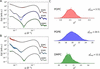
Fig. 3 shows the best fits for POPC-, POPE- and DMPC-based LUV samples. The data are compared with model curves generated using the median values of each adjustable parameter distribution (Fig. 3A). These `median curves' are in turn compared with the outcomes of individual iterations (Fig. 3B), highlighting which q ranges are most affected by data uncertainties and parameter distribution widths. Additionally, the stochastic nature of the minimization algorithm is reflected in the distribution profiles in Fig. 3C. The adaptive convergence criteria enable a compact distribution, with a relative discrepancy between minimum and maximum values of approximately 30% (POPC), 50% (POPE) and 20% (DMPC). In the cases of POPC and POPE, the large variations in values are primarily due to uncertainties in the LUV size ( ), as highlighted in the very low q range in Fig. 3B. In the case of POPE, the variability is further exacerbated by current model inconsistencies in describing the intensity minimum in the range q = 0.02–0.03 Å−1, likely affected by the bilayer bending fluctuations [see e.g. Chappa et al. (2021) and Milner & Safran (1987)].
|
Figure 3
Best fits of POPC (red), POPE (blue) and DMPC (green) LUV SAXS data with  . (A) Black lines display the model as a function of the parameter medians. These are compared with the best fits of each iteration in (B), where the shade of color reflects the best values (brighter for low values, darker for high values). (C) Distributions of values.  values were calculated using the adjustable parameter medians. Smooth curves display the kernel density estimates (KDEs) of the underlying histograms. |
The results for the adjustable parameters are summarized in Table 3 for POPC LUVs, along with a comparison with previous results reported by Kučerka et al. (2011) and Frewein et al. (2021). The results and comparison for POPE and DMPC are provided in Tables S3 and S5. Note that our results are reported as median values and MADs. For reference, for a normal distribution, the relationship between standard deviation and MAD is  .
‡Fixed values. §`Soft' Bayesian constrains (Kučerka et al., 2011 ).
|
||||||||||||||||||||||||||||||||||||||||||||||||||||||||||||||||||||||||||||||||||||||||||||||||||||||||||||||||||||||||||||||||||||||||||||||||||||||||||||||
 MAD and compared with previous results. Number of iterations


















 C)

 (Å


 (Å)


 (Å)


 (Å)


 (Å


 (Å)
 (Å)
 (Å)

It is important to note a methodological difference when comparing our results with the reference studies by Kučerka et al. (2011) (PC species) and Kučerka et al. (2015) (PE species). In those studies, vesicles were prepared by extrusion through 50 nm filters, yielding small unilamellar vesicles (SUVs), whereas our analysis is based on 100 nm LUVs. The higher membrane curvature of SUVs compared with LUVs can induce a weak but systematic membrane thinning (Chappa et al., 2021). In addition, the reference systems were analyzed over a more restricted q range ( Å
 ) using a joint SAXS/SANS analysis approach. Despite these differences in vesicle size, q range and overall analysis methodology our results demonstrate remarkable agreement with the earlier findings. This consistency, on the one hand, suggests that curvature effects are negligible for POPC and POPE under the conditions considered and, on the other hand, highlights the robustness of the SAS_MoCa minimization engine in delivering reliable parameter estimates and confidence intervals, even with a relatively large number of adjustable parameters.
For DMPC, we faced a specific challenge regarding prior knowledge. While structural parameters for POPC and POPE lipids are well documented in the literature, information regarding the hydration layer volume,  , and the acyl-chain thickness fluctuation width,
 , for DMPC was unavailable. Consequently, for the DMPC analysis, we adopted broad, non-informative rectangular priors (hard boundaries) for and . Remarkably, even without informative priors for these parameters, the TSA algorithm converged to physically meaningful values (Table S5), demonstrating the robustness of the minimization engine even for under-constrained parameters.
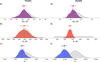
In addition to reporting point estimates, the full strength of the Bayesian framework implemented in SAS_MoCa lies in inspecting the posterior distributions of the adjustable parameters, their correlations and their relationship to the chosen priors. Fig. 4 shows the posterior probability densities of selected parameters together with their corresponding prior distributions. These posterior distributions constitute the primary output of the program and should always be examined before interpreting the associated median and MAD values. The parameters in Figs. 4A and 4B illustrate cases where the posteriors remain closely aligned with their priors. By contrast, the distributions in Figs. 4C, 4D and 4F exhibit a clear shift in center of mass relative to the prior mean, exemplifying data-driven updating of informative priors. Fig. 4E shows a similar data-driven update but starting from a non-informative prior. The full set of posterior results for all adjustable parameters is provided in Figs. S2–S4.
|
Figure 4
Comparison between probability density distributions (posteriors) and priors of three selected adjustable parameters obtained during the curve fitting of POPC (A–C) and POPE systems (D–F). (A, D) Acyl-chain thickness  ; (B, E) vesicle radius ; and (C, F) relative variation of acyl-chain thickness  . The histograms contain entries; colored curves represent KDEs, while dotted black lines show the associated prior distribution. Symbols with error bars highlight the median and MAD values for each probability distribution. |
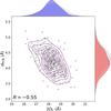
On the basis of the found posterior distributions, the program automatically generates a heatmap representing the matrix of Pearson correlation coefficients for the adjustable parameters. Fig. 5 shows a selected example of the correlation between adjustable parameters. Full correlation matrices for POPC, POPE and DMPC systems are shown in Figs. S5–S7.
|
Figure 5
KDE bivariate density map and associated probability densities of two selected adjustable parameters obtained during the curve fitting of POPC systems: acyl-chain thickness (blue, x axis) and distance between PCN and CG quasi-molecular groups  (red, y axis). Results from iterations. Dashed gray lines indicate the associated prior distribution. R is the Pearson correlation coefficient. |
4.2. Benchmarking parameter sensitivity and prior choices
We investigated how priors affect both sensitive and non-sensitive adjustable parameters. To this end, we reanalyzed the POPC data while systematically modifying the prior by one parameter at a time. Specifically, we shifted the prior mean in steps of  and examined the resulting posterior distribution of the corresponding parameter y.
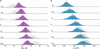
As illustrated in Fig. 6 for two representative parameters, we observed two characteristic behaviors. Fig. 6A shows a sensitive parameter, the acyl-chain thickness  . Here, the posterior is dominated by the likelihood and remains largely unchanged when the prior is shifted, indicating that the data strongly constrain . In contrast, Fig. 6B shows a non-sensitive parameter, the lipid head-group volume
 . In this case, the posterior distributions closely track the shifted priors, demonstrating that the posterior is prior-dominated and essentially determined by the initial belief—even when that belief corresponds to non-physical values.
|
Figure 6
Verifying the dependency of parameter distributions on priors: sensitive versus non-sensitive parameters. (A) Acyl-chain thickness distributions (KDE representation in purple) against priors shifted by  (gray). (B) Lipid head-group volume  distributions (KDE representation in blue) against priors shifted by (gray). Vertical dashed lines indicate the medians of the adjustable parameter distributions. Number of iterations for each independent analysis  . |
Even for sensitive parameters such as , the choice of prior can induce a noticeable shift in the posterior median. Users should therefore exercise care when specifying priors: the principle of `garbage in, garbage out' applies, and the reliability of the inferred parameters depends critically on the quality and physical plausibility of the prior information.
4.3. Reproducibility and practical guidelines
Accessing the sampling distributions of each adjustable parameter enables the application of basic statistical inference tools. In particular, we can utilize these distributions to verify the consistency of results across independent analyses performed with varying numbers of iterations,  . For normal-like (i.e. symmetric, bell-shaped) distributions, the median is comparable to the mean,
 , and the standard deviation is approximated by
 . Consequently, one can estimate the confidence intervals (CIs) for both and
 using the pivotal method (Ramachandran & Tsokos, 2015). Specifically, the
 CIs for the mean as
 are given by

where α is the significance level,  represents the critical values of the Student t distribution with
 degrees of freedom and
 denotes the corresponding quantiles of the standard normal distribution for large sample sizes (Ramachandran & Tsokos, 2015).
Similarly, the CIs for the variance  are

where  are the critical values of the -distribution tails (Ramachandran & Tsokos, 2015).
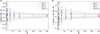
Fig. 7 illustrates the reproducibility of results for varying and compares the empirical distributions with predicted CIs. The latter are calculated by averaging the and outcomes for as references for equations (7) and (8). As shown in Fig. 7A, the distributions of the medians are well contained within the predicted confidence intervals. However, for the standard deviations (Fig. 7B), the empirical spread appears larger than the theoretical prediction, particularly for small . This is probably because, e.g., the posterior distributions are not perfectly normal.
|
Figure 7
Median (A) and equivalent standard deviation (B) values from independent analyses performed at different values. Lines mark the ranges for different levels of CIs. These are calculated using equations (7) (A) and (8) (B), by using the average of the outcomes for as and values. |
These reproducible behaviors inform a recommended workflow for SAS_MoCa users:
(1) Exploratory phase. Perform rapid tests with a small number of iterations ( –20) and varied initializations to assess parameter sensitivity, validate posterior results and refine prior choices.
(2) Precision planning. Invert equations (7) and (8) and use preliminary results to estimate the required to achieve a target confidence interval width, optimizing computational resources.
(3) Conclusive analysis. Execute a computationally intensive run with, e.g.,  to generate robust posterior distributions, once the model initialization is validated.
This tiered approach ensures that computational effort is allocated efficiently, balancing rapid feedback with statistical rigor.
5. Conclusion
We have presented SAS_MoCa, an open-source computational framework designed to address a critical bottleneck in the structural characterization of LUVs via small-angle X-ray scattering. To our knowledge, SAS_MoCa represents the first freely available software capable of performing compositional scattering density profile analysis tailored specifically for LUVs, filling a significant gap left by discontinued proprietary tools and general-purpose packages lacking specialized workflows for membrane compositional modeling.
The core innovation of SAS_MoCa lies in its rigorous application of Bayesian inference to SAXS data analysis. By integrating adaptive thermodynamic simulated annealing with flexible prior probability distributions, the software enables robust statistical quantification of parameter uncertainties and correlations, even in highly under-constrained regimes typical of single-curve scattering experiments. This approach fundamentally shifts the analytical workflow from heuristic trial-and-error fitting to transparent statistical inference. Users are no longer forced to accept point estimates without context; instead, the explicit comparison of prior and posterior distributions provides a diagnostic view of which structural parameters are truly resolved by the experimental data and which remain constrained by external knowledge.
Our validation across three distinct lipid systems—POPC, POPE and DMPC—demonstrates that SAS_MoCa yields results consistent with established joint SAXS/SANS literature, despite analyzing single-curve datasets with significantly higher degrees of freedom. Crucially, the benchmarking of parameter sensitivity highlights the necessity of physically meaningful priors: while the minimization engine is robust, the reliability of the posterior remains bounded by the validity of the initial assumptions. This feature enforces a higher standard of scrutiny, requiring researchers to explicitly justify their structural hypotheses rather than relying on implicit constraints within black-box algorithms.
Looking ahead, the modular architecture of SAS_MoCa is designed for extensibility. Current development efforts aim to incorporate multiscale models for proteoliposomes and extend the formalism to handle small-angle neutron scattering, including joint contrast-variation analyses. Furthermore, we plan to expand the library of compositional models to cover more complex compositions—including cholesterol or drugs [see, e.g., Pachler et al. (2019)], asymmetric LUVs, bacterial systems (Semeraro et al., 2017; Semeraro et al., 2021), and minimal cells—thereby broadening the applicability of the framework to increasingly complex biomimetic membrane systems.
SAS_MoCa is released under the BSD 3-Clause license and is publicly available at https://github.com/PabstLab/SAS_MoCa (Semeraro & Pabst, 2026). We envision SAS_MoCa democratizing high-resolution membrane structural analysis—empowering laboratories to perform rigorous, compositional investigations with full statistical transparency. By making advanced Bayesian inference accessible to the broader biophysics community, the tool fosters a culture of reproducible reporting where assumptions are explicit and uncertainties are quantified.
APPENDIX A
Scattering intensity
A1. Vesicle size and polydispersity: separated form factor model
In the SFF framework the LUV's shape is described by an infinitesimally thin spherical frame of radius  . The radius polydispersity is described by the Schulz probability distribution function, which ensures an analytical form (Pencer et al., 2006). The scattering intensity of such a two-dimensional, polydisperse set of spherical frames is given by
 , where

Here  , and Z is the width parameter of the Schulz distribution [the variance is defined as
 ]. Note that
 , where
 is the spherical Bessel function of zeroth order.
The limit for zero scattering angle (forward scattering) is

A2. Transbilayer structure: scattering density profile
The scattering amplitude for the transbilayer structure of lipid bilayers, , refers to the latest update of the SDP model (Frewein et al., 2021). The SDP approach is a compositional model that takes into account the chemical compositions of quasi-molecular groups in which the lipids are parsed. Therefore, the specific scattering amplitude contribution depends on the lipid composition. In the following, we describe the basic models pertaining to the quasi-molecular parsing of POPC, POPE and DMPC, as described by Kučerka et al. (2011), Kučerka et al. (2015) and Frewein et al. (2021).
The base scattering amplitude is given by
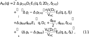
where the functions


are the Fourier transform of a Gaussian profile (12) and an error-function-based smooth rectangular profile (13). The subscript j refers to the chain quasi-molecular group CH3 and CH; the subscript k includes the lipid head groups (e.g. CG, PCN and cholCH3 in the case of POPC; see supporting information). For the generic ith quasi-molecular group the parameter
zi is the center of the Gaussian or smooth rectangular functions;  is the associated width of either the Gaussian profile or the error functions composing the smooth rectangular profile. In the latter case the distance between the centers of the two error functions is
Li.
The acyl-chain thickness fluctuation average, , is accounted for with the expression

where  is the Gaussian probability distribution function of mean
 and standard deviation
 (Frewein et al., 2021).
The parameters describing  are described and listed in Table 4. For details refer to Frewein et al. (2021) and Kučerka et al. (2008).
|
||||||||||||||||||||||||||||||||||||||||||||||||||


 Å


Supporting information
Supplementary Information. DOI: https://doi.org/10.1107/S1600576726009180/ge5187sup1.pdf
Acknowledgements
We thank the BM29 beamline staff at the ESRF (Grenoble, France) for support during beamtime (proposal No. MX-2282). We thank Paulina Piller for help in sample preparation; Moritz Frewein for the fruitful discussion; and Shahrzad Dabironezare for testing the repository and identifying bugs. Open access funding provided by Universitat Gräz.
Conflict of interest
The authors declare no conflict of interest.
Data availability
Data and example scripts used in this study are openly available in the examples directory of the SAS_MoCa GitHub repository: https://github.com/PabstLab/SAS_MoCa.
Funding information
This project has received funding from the European Union's Horizon Europe research and innovation programme under grant agreement No. 101169269. This research was funded in whole or in part by the Austrian Science Fund (FWF) (10.55776/PIN7380924).
References
 Chacko, I. A., Ghate, V. M., Dsouza, L. & Lewis, S. A. (2020). Colloids Surf. B Biointerfaces 195, 111262.
CrossRef
PubMed
Google Scholar
Chappa, V., Smirnova, Y., Komorowski, K., Müller, M. & Salditt, T. (2021). J. Appl. Cryst. 54, 557–568.
Web of Science
CrossRef
CAS
IUCr Journals
Google Scholar
de Vicente, J., Lanchares, J. & Hermida, R. (2003). Phys. Lett. A 317, 415–423.
CrossRef
CAS
Google Scholar
Frewein, M. P., Piller, P., Semeraro, E. F., Czakkel, O., Gerelli, Y., Porcar, L. & Pabst, G. (2023). Biophys. J. 122, 2445–2455.
CrossRef
CAS
PubMed
Google Scholar
Frewein, M. P. K., Doktorova, M., Heberle, F. A., Scott, H. L., Semeraro, E. F., Porcar, L. & Pabst, G. (2021). Symmetry 13, 1441.
CrossRef
PubMed
Google Scholar
Frewein, M. P. K., Rumetshofer, M. & Pabst, G. (2019). J. Appl. Cryst. 52, 403–414.
CrossRef
CAS
IUCr Journals
Google Scholar
Harris, C. R., Millman, K. J., van der Walt, S. J., Gommers, R., Virtanen, P., Cournapeau, D., Wieser, E., Taylor, J., Berg, S., Smith, N. J., Kern, R., Picus, M., Hoyer, S., van Kerkwijk, M. H., Brett, M., Haldane, A., del Río, J. F., Wiebe, M., Peterson, P., Gérard-Marchant, P., Sheppard, K., Reddy, T., Weckesser, W., Abbasi, H., Gohlke, C. & Oliphant, T. E. (2020). Nature 585, 357–362.
Web of Science
CrossRef
CAS
PubMed
Google Scholar
Harvey, A. H. (1998). Thermodynamic Properties of Water: Tabulation from the lAPWS Formulation 1995 for the Thermodynamic Properties of Ordinary Water Substance for General and Scientific Use. NIST Interagency/Internal Report (NISTIR), National Institute of Standards and Technology, Gaithersburg, MD, USA.
Google Scholar
Hunter, J. D. (2007). Comput. Sci. Eng. 9, 90–95.
Web of Science
CrossRef
Google Scholar
Konarev, P. V., Gruzinov, A. Y., Mertens, H. D. T. & Svergun, D. I. (2021). J. Appl. Cryst. 54, 169–179.
Web of Science
CrossRef
CAS
IUCr Journals
Google Scholar
Krzywon, J., Adams, M., Agouzal, N., Alina, G., Attala, Z., Backman, M., Bakker, J., Beaucage, P., Berger, J., Bourne, R., Bouwman, W., Bressler, I., Butler, P., Cadwallader-Jones, I., Campbell, K., Cho, J.-H., Cooper-Benun, T., Cortes Hernandez, R., Crake-Merani, J. A., Detiste, A., Doucet, M., Doutch, J., Dresen, D., Drosos, G., Durniak, C., Farrow, C., Ferraz Leal, R., Ford, R., Forster, L., Gaudet, J., Gerina, M., Gilbert, P., Gonzalez, M., Hammond, O., Hansen, T. B., Heenan, R., Henson, S., Hewins, E., Hicks, A., Honecker, D., Jackson, A., Jensen, G., Juhas, P., Karliczek, J., Kienzle, P., King, S., Kline, S., Lin, J., Liu, Y., Lopes, R., Lozano, D., Lytje, K., Mannicke, D., Maranville, B., Markvardsen, A., Martinez, N., McKerns, M., Miller, B., Mothander, K., Murphy, R., Nelson, A., Nielsen, T., O'Driscoll, L., Oakley, M., Park, H., Parker, P., Patrou, M., Peterson, P., Potrzebowski, W., Prescott, S., Rakitin, M., Richter, T., Rooks, J., Rozyczko, P., Shan, X., Sharp, P., Shrestha, S., Snow, T., Stellhorn, A., Teixeira, S., Tumarkin, J., Washington, A., Weigandt, K., Whitley, R., Wilkins, L., Wolf, C., Zhang, A. & Zheng, A. (2025). SasView. Version 6.1.2. https://doi.org/10.5281/zenodo.17795298.
Google Scholar
Kučerka, N., Nagle, J. F., Sachs, J. N., Feller, S. E., Pencer, J., Jackson, A. & Katsaras, J. (2008). Biophys. J. 95, 2356–2367.
Web of Science
PubMed
Google Scholar
Kučerka, N., Nieh, M.-P. & Katsaras, J. (2011). Biochim. Biophys. Acta 1808, 2761–2771.
PubMed
Google Scholar
Kučerka, N., van Oosten, B., Pan, J., Heberle, F. A., Harroun, T. A. & Katsaras, J. (2015). J. Phys. Chem. B 119, 1947–1956.
PubMed
Google Scholar
Lewis-Laurent, A., Doktorova, M., Heberle, F. A. & Marquardt, D. (2021). Biophys. J. 120, 4639–4648.
CAS
PubMed
Google Scholar
McKerns, M., Strand, L., Sullivan, T., Fang, A. & Aivazis, M. A. G. (2012). arXiv, 1202.1056[cs. MS].
Google Scholar
McKinney, W. (2010). Proceedings of the 9th Python in Science Conference, pp. 56–61. SciPy.
Google Scholar
Milner, S. T. & Safran, S. A. (1987). Phys. Rev. A 36, 4371–4379.
CrossRef
CAS
Google Scholar
Nagle, J. F., Venable, R. M., Maroclo-Kemmerling, E., Tristram-Nagle, S., Harper, P. E. & Pastor, R. W. (2019). J. Phys. Chem. B 123, 2697–2709.
CrossRef
CAS
PubMed
Google Scholar
Pabst, G., Koschuch, R., Pozo-Navas, B., Rappolt, M., Lohner, K. & Laggner, P. (2003). J. Appl. Cryst. 36, 1378–1388.
Web of Science
CrossRef
CAS
IUCr Journals
Google Scholar
Pabst, G., Kučerka, N., Nieh, M.-P. & Katsaras, J. (2014). Editors. Liposomes, Lipid Bilayers and Model Membranes: From Basic Research to Application. Boca Raton: CRC Press.
Google Scholar
Pabst, G., Rappolt, M., Amenitsch, H. & Laggner, P. (2000). Phys. Rev. E 62, 4000–4009.
CrossRef
CAS
Google Scholar
Pachler, M., Kabelka, I., Appavou, M.-S., Lohner, K., Vácha, R. & Pabst, G. (2019). Biophys. J. 117, 1858–1869.
CrossRef
CAS
PubMed
Google Scholar
Pan, J., Heberle, F. A., Tristram-Nagle, S., Szymanski, M., Koepfinger, M., Katsaras, J. & Kučerka, N. (2012). Biochim. Biophys. Acta 1818, 2135–2148.
CrossRef
CAS
PubMed
Google Scholar
Pencer, J., Krueger, S., Adams, C. P. & Katsaras, J. (2006). J. Appl. Cryst. 39, 293–303.
Web of Science
CrossRef
CAS
IUCr Journals
Google Scholar
Ramachandran, K. M. & Tsokos, C. P. (2015). Mathematical Statistics with Applications in R. Academic Press.
Google Scholar
Scott, H. L., Skinkle, A., Kelley, E. G., Waxham, M. N., Levental, I. & Heberle, F. A. (2019). Biophys. J. 117, 1381–1386.
Web of Science
CrossRef
CAS
PubMed
Google Scholar
Semeraro, E., Frewein, M. P. K. & Pabst, G. (2024). Methods Enzymol. 700, 349–383.
CAS
PubMed
Google Scholar
Semeraro, E. F., Devos, J. M., Porcar, L., Forsyth, V. T. & Narayanan, T. (2017). IUCrJ 4, 751–757.
CrossRef
CAS
PubMed
IUCr Journals
Google Scholar
Semeraro, E. F., Marx, L., Mandl, J., Frewein, M. P. K., Scott, H. L., Prévost, S., Bergler, H., Lohner, K. & Pabst, G. (2021). J. Appl. Cryst. 54, 473–485.
CrossRef
CAS
IUCr Journals
Google Scholar
Semeraro, E. F. & Pabst, G. (2026). SAS_MoCa. Version 1.5.0. https://github.com/PabstLab/SAS_MoCa.
Google Scholar
The pandas development team (2020). pandas-dev/pandas: Pandas,https://doi.org/10.5281/zenodo.3509134.
Google Scholar
Tully, M. D., Kieffer, J., Brennich, M. E., Cohen Aberdam, R., Florial, J. B., Hutin, S., Oscarsson, M., Beteva, A., Popov, A., Moussaoui, D., Theveneau, P., Papp, G., Gigmes, J., Cipriani, F., McCarthy, A., Zubieta, C., Mueller-Dieckmann, C., Leonard, G. & Pernot, P. (2023). J. Synchrotron Rad. 30, 258–266.
Web of Science
CrossRef
IUCr Journals
Google Scholar
Virtanen, P., Gommers, R., Oliphant, T. E., Haberland, M., Reddy, T., Cournapeau, D., Burovski, E., Peterson, P., Weckesser, W., Bright, J., van der Walt, S. J., Brett, M., Wilson, J., Millman, K. J., Mayorov, N., Nelson, A. R. J., Jones, E., Kern, R., Larson, E., Carey, C. J., Polat, I., Feng, Y., Moore, E. W., VanderPlas, J., Laxalde, D., Perktold, J., Cimrman, R., Henriksen, I., Quintero, E. A., Harris, C. R., Archibald, A. M., Ribeiro, A. H., Pedregosa, F., van Mulbregt, P., Vijaykumar, A., Bardelli, A. P., Rothberg, A., Hilboll, A., Kloeckner, A., Scopatz, A., Lee, A., Rokem, A., Woods, C. N., Fulton, C., Masson, C., Häggström, C., Fitzgerald, C., Nicholson, D. A., Hagen, D. R., Pasechnik, D. V., Olivetti, E., Martin, E., Wieser, E., Silva, F., Lenders, F., Wilhelm, F., Young, G., Price, G. A., Ingold, G., Allen, G. E., Lee, G. R., Audren, H., Probst, I., Dietrich, J. P., Silterra, J., Webber, J. T., Slavič, J., Nothman, J., Buchner, J., Kulick, J., Schönberger, J. L., de Miranda Cardoso, J. V., Reimer, J., Harrington, J., Rodríguez, J. L. C., Nunez-Iglesias, J., Kuczynski, J., Tritz, K., Thoma, M., Newville, M., Kümmerer, M., Bolingbroke, M., Tartre, M., Pak, M., Smith, N. J., Nowaczyk, N., Shebanov, N., Pavlyk, O., Brodtkorb, P. A., Lee, P., McGibbon, R. T., Feldbauer, R., Lewis, S., Tygier, S., Sievert, S., Vigna, S., Peterson, S., More, S., Pudlik, T., Oshima, T., Pingel, T. J., Robitaille, T. P., Spura, T., Jones, T. R., Cera, T., Leslie, T., Zito, T., Krauss, T., Upadhyay, U., Halchenko, Y. O. & Vázquez-Baeza, Y. (2020). Nat. Methods 17, 261–272.
Web of Science
CrossRef
CAS
PubMed
Google Scholar
This is an open-access article distributed under the terms of the Creative Commons Attribution (CC-BY) Licence, which permits unrestricted use, distribution, and reproduction in any medium, provided the original authors and source are cited.
| JOURNAL OF APPLIED CRYSTALLOGRAPHY |