Bridging the small-angle X-ray scattering–X-ray diffraction gap in disordered layered materials: the CLADIFFMOD unified framework

A unified multi-scale model is presented for the simultaneous description of small-angle X-ray scattering (SAXS) and X-ray diffraction (XRD) in disordered 2:1 clay minerals, providing a computationally tractable approximation that bridges the two analytical traditions under the tested experimental conditions. The total scattered intensity is expressed as a continuous physically consistent function of the scattering vector magnitude, decomposed into three physically distinct contributions: a polydisperse disc form factor governing the SAXS regime, a Monte Carlo implementation of the Drits–Tchoubar Markov-chain stacking model for basal 00l reflections and a Debye equation turbostratic scattering term for in-plane hkl correlations. The three contributions are coupled through a sigmoid crossover approximation designed to provide a continuous transition between morphology-dominated and stacking-dominated scattering regimes. The crossover amplitude is measured directly from the experimental data and constitutes the primary coupling observable between morphological and crystallographic length scales. A critical innovation over existing approaches is the treatment of intra-stack heterogeneity: stacking sequences are generated layer by layer via a first-order Markov chain with transition matrix T. The model is validated against five experimental datasets acquired on an Na-montmorillonite reference under controlled relative humidity conditions. The framework is implemented in the open Python code CLADIFFMOD and is directly transferable to any 2:1 disordered clay mineral by substitution of the hydration-state dictionary and the Markov transition matrix.

1. Introduction

1.1. Clay mineral structural disorder: a multi-scale challenge

Smectite clay minerals are among the most structurally complex naturally occurring materials. Their fundamental building block, the 2:1 (tetrahedral–octahedral–tetrahedral, TOT) layer, is itself well understood: an octahedral sheet of Al³⁺ or Mg²⁺ cations sandwiched between two tetrahedral Si–O sheets, with isomorphous substitutions generating a permanent layer charge that is compensated by exchangeable interlayer cations and water molecules (Odom, 1984; Kloprogge et al., 1999; Oueslati et al., 2009; Ammar et al., 2014; Oueslati & Meftah, 2018; Mejri et al., 2023a). The structural complexity arises at the supramolecular scale, where the stacking of successive layers produces a three-dimensional disordered architecture that is not periodic in the crystallographic sense and therefore cannot be described by classical space-group symmetry (Johnston, 2010; Gilbert et al., 2015; Ferrage, 2016; Loganathan et al., 2020; Oueslati & Meftah, 2026).

Two types of disorder coexist in smectite systems. Stacking disorder (the irregular succession of hydration states, the variable orientation of adjacent layers and the distribution of interlayer spacing) produces broad, asymmetric and sometimes extinct basal 00l reflections that are the primary fingerprint of clay hydration and interstratification. Morphological disorder (polydispersity in platelet lateral dimensions, thickness and aggregation state) governs the small-angle scattering behaviour and controls the colloidal and rheological properties of clay suspensions (Besson et al., 1974; Brindley, 1980; Pons, 1980; Vali & Köster, 1986; Lanson & Besson, 1992; Ahn & Buseck, 1990; Drits, 1997; Środoń, 1999; Plançon, 2001; Drits, 2003; Guyonnet et al., 2005; Guggenheim, 2011; Brigatti & Mottana, 2011; Lanson, 2011; Gilbert et al., 2015; Mejri et al., 2021; Oueslati et al., 2022). Although these two types of disorder are physically inseparable – they coexist within the same particle, and the coherent domain size M governs both the width of the 001 reflection and the Guinier knee of the small-angle signal – they have been analysed independently for more than half a century, using fundamentally different formalisms, instruments and software (Plançon & Tchoubar, 1977; Reynolds, 1993; Plançon, 2002; Sakharov et al., 2004; Lanson, 2005; Tchoubar & Cohaut, 2006; Britto et al., 2010; Gilbert et al., 2015; Hamley, 2022; Chaaya et al., 2023; Marangoni & Pensini, 2026).

This methodological separation constitutes the central unresolved problem addressed by the present work: the small-angle X-ray scattering (SAXS)–X-ray diffraction (XRD junction. The first-order 001 basal reflection of an Na-smectite in the 1W hydration state falls at q₀₀₁ ≃ 0.51 Å⁻¹ (d₀₀₁ ≃ 12.3 Å; 2θ ≃ 7.2° with Cu Kα radiation), directly at the boundary between the small-angle (SAXS) and wide-angle (XRD) analysis domains. No prior model has been able to treat this reflection coherently within a single framework that simultaneously accounts for particle morphology and stacking periodicity. The consequence is a systematic inconsistency in the derived structural parameters: the coherent domain size, the hydration state fractions and the interstratification degree are determined independently from SAXS and XRD, without any mutual constraint, and the two sets of parameters are rarely consistent.

1.2. X-ray diffraction analysis of disordered clays

The theoretical foundations for the quantitative analysis of disordered clay mineral diffractograms were established by Méring (1949), who demonstrated that the intensity distribution of basal reflections from randomly interstratified clay minerals could be expressed as a function of layer-pair probabilities. This framework was subsequently formalized by Drits & Tchoubar (1990) into a rigorous matrix formalism, the most complete and physically exact treatment of 00l scattering from disordered lamellar structures available in the literature, in which the intensity is expressed as

where F_i(q) and F_j(q) are the structure factors of layers of types i and j, respectively; the asterisk denotes complex conjugation. W_ij is the probability of occurrence of layer pairs of types i and j, and R_ij(q) is the interference function. Computer implementations of this formalism, most notably NEWMOD (Reynolds, 1985) and the Fortran code AB2F (Plançon & Drits, 2000; Plançon, 2002), have become standard tools for the quantitative mineralogical analysis of interstratified clay minerals and remain in widespread use.

Subsequent decades saw considerable refinement of this framework, particularly through the contributions of Drits and Sakharov, who systematically explored the effects of stacking disorder on reflection profiles, and of Lanson and colleagues, who extended the formalism to mixed-layer systems under variable humidity and ionic strength conditions (Bookin et al., 1989; Plançon & Zacharie, 1990; Drits et al., 1993; Drits et al., 1997; Ferrage et al., 2005; Lanson et al., 2009; Sakharov & Drits, 2015; Sakharov et al., 2016). Besson & Drits (1997) provided a comprehensive treatment of layer charge heterogeneity and its influence on diffraction patterns, while Plançon (2002) addressed the statistical equivalence between Markov-chain descriptions of interstratification and the matrix formalism of Drits & Tchoubar (1990). These studies collectively established the XRD analysis of disordered clays as a mature discipline. Nevertheless, all of these approaches share a fundamental limitation: they are defined exclusively over the wide-angle domain (q ≥ 0.5 Å⁻¹) and carry no information on particle morphology. More recent investigations by Oueslati and colleagues (Oueslati et al., 2009; Oueslati et al., 2012; Oueslati et al., 2015; Mejri et al., 2023b; Oueslati & Meftah, 2026; Oueslati, 2026a) have demonstrated that the quantitative analysis of smectite hydration sequences requires accounting for the full complexity of interstratification, including the coexistence of multiple hydration states within a single coherent domain – a point that has critical implications for the construction of physically realistic stacking models, as we discuss below.

1.3. Small-angle scattering of clay minerals

The analysis of SAXS data from clay mineral suspensions and gels has developed independently from the XRD tradition, drawing primarily on colloid science and polymer physics formalisms. Platelet form factors (disc, lamella, cylinder) fitted to the Guinier and Porod regimes provide estimates of the lateral diameter L, the thickness t, and the fractal or compact character of clay aggregates (Anovitz & Weston, 2020).

A key parameter extracted from both SAXS and XRD analyses is the coherent domain size M – the number of layers contributing to a single coherent scattering event (Jensen et al., 2006; Giannini et al., 2016). From the XRD perspective, M controls the width and shape of basal reflections through the Debye–Scherrer relationship and its disordered-lattice generalizations (Lele & Anantharaman, 1966; Basak et al., 2022). From the SAXS perspective, Md₀₀₁ determines the platelet thickness, which sets the position of the crossover between the Guinier and Porod regimes. In principle, these two independent determinations of M from the same sample should yield identical values. In practice, they rarely do – a discrepancy that has been noted but not resolved (Beaucage, 1995; Hammouda, 2010; Singh, 2017).

The root cause of this discrepancy is the absence of a unified model. Because SAXS and XRD analyses use different experimental setups, different data reduction procedures and different fitting formalisms, the resulting structural parameters are not mutually consistent. The 001 reflection, which carries joint information on both the morphological (thickness) and crystallographic (hydration state, interstratification) properties of the clay, falls in the gap between the two analysis domains and is therefore not optimally exploited by either approach.

1.4. The SAXS–XRD junction

The failure to bridge the SAXS and XRD domains is not a consequence of insufficient experimental data or inadequate computing resources. It reflects a deeper conceptual limitation: the two analysis traditions were built on different physical approximations that are mutually incompatible at the junction.

On the XRD side, classical approaches treat the clay as an infinite (or semi-infinite) periodic lattice with stochastic substitutions, ignoring particle boundaries. On the SAXS side, form factor models treat the platelet as a finite object with well defined surfaces, ignoring internal crystallographic periodicity. The junction zone, q ≃ 0.3–0.7 Å⁻¹, is the region where both the periodicity and the finite size of the platelet contribute comparably to the scattered intensity. It is precisely in this zone that the 001 reflection lies and both models fail. Several partial attempts have been made to address this problem. Ramsay & Lindner (1993), Classen et al. (2013), and Pabst and colleagues (Heftberger et al., 2014; Frewein et al., 2019; Pabst & Blochowicz, 2022) noted the inconsistency between SAXS-derived and XRD-derived thickness estimates but attributed it to sample preparation artefacts rather than to a modelling deficiency. Dabat and colleagues (Hu et al., 2011; Dabat et al., 2020) combined SAXS and ²H NMR to constrain platelet dimensions but did not attempt a unified scattering model. To the best of our knowledge, few studies have attempted to combine particle morphology, interstratified stacking disorder, turbostratic scattering and the SAXS–XRD crossover within a single modelling framework for disordered clay minerals. Previous investigations of related lamellar systems, including those of Heftberger et al. (2014) and Marangoni & Pensini (2026), addressed important aspects of multi-scale scattering in layered materials but did not specifically consider the combined treatment of platelet morphology, Markovian interstratification, turbostratic scattering or hydration-state disorder in expandable 2:1 clay minerals.

1.5. A unified multi-scale formulation

In this work, we present a unified model for the full X-ray scattering signal of disordered 2:1 clay minerals, spanning the range q ∈ [0.1, 5.5] Å⁻¹ (approximately 2θ ∈ [0.8°, 60°] for Cu Kα radiation). The model decomposes the total scattered intensity into three physically distinct contributions, each associated with a characteristic structural length scale:

(i) The SAXS contribution (q ≤ 0.4 Å⁻¹), which describes particle morphology through a polydisperse disc form factor. This contribution constrains the platelet lateral dimensions and the Guinier regime.

(ii) The 00l contribution (q ≥ 0.4 Å⁻¹), which describes stacking order through a Monte Carlo implementation of the Drits–Tchoubar Markov-chain formalism.

(iii) The turbostratic hkl contribution (q ≥ 0.6 Å⁻¹), which describes the continuous background between basal reflections arising from in-plane atomic correlations.

The three contributions are coupled through a continuous sigmoid weighting function that provides a smooth differentiable transition across the junction zone. The amplitude of the XRD contribution at the junction is fixed by the directly measurable ratio I_exp(001)/I_max(SAXS) – a quantity that encodes the relative importance of stacking periodicity versus particle morphology at the crossover scattering vector magnitude, and that constitutes the key coupling parameter between the two analytical traditions.

The model is implemented in the open Python code CLADIFFMOD and operates in two modes: a full SAXS + XRD mode for datasets covering the complete q range, and an XRD-only mode for conventional diffractograms (2θ = 3°–60°). In both modes, all structural parameters carry a direct physical interpretation (Table 1) and can in principle be constrained by independent measurements.

2. Model description

2.1. The SAXS–XRD junction: the central unresolved problem

The historical motivation and scientific context of the SAXS–XRD junction problem were introduced in Section 1. Here, we focus exclusively on the mathematical formulation adopted in the present work. The total scattering intensity is represented as the combination of morphology-dominated, stacking-dominated and turbostratic contributions, as de­scribed below (Shang et al., 2003; Leu et al., 2016; Birmpilis et al., 2019a; Birmpilis et al., 2019b).

2.2. General formulation of the unified intensity

The present model expresses the total scattered intensity as a physically motivated superposition of three contributions, each associated with a characteristic structural length scale:

The central coupling element is the continuous weighting function w(q), which controls the transition between the SAXS-dominated and XRD-dominated regimes. This function, rather than a hard boundary, is the architectural solution to the junction problem. Its definition and physical justification are given in Section 2.5.

2.3. Basal reflections and Markovian intra-stack heterogeneity

2.3.1. Layer structure factor

The layer structure factor F_layer(q) is computed by explicit summation over all atomic sites projected onto the stacking axis, following the dynamic atomic total form factor scheme (DATFS) of Bailey (1988) for dioctahedral smectite [Si₄Al_1.67Mg_0.33O₁₀(OH)₂]:

Here n_j, f_j(s), B_j and z_j are, respectively, the site multiplicity, the atomic scattering factor (Waasmaier & Kirfel, 1995), the isotropic Debye–Waller factor and the axial coordinate of site j; s = q/(4π) = sin(θ)/λ (Poiarkova & Rehr, 1999). The layer structure factor formulation is validated by the systematic extinction of the 002 reflection, which arises from destructive interference between the two tetrahedral sheets and constitutes an unambiguous structural fingerprint of well ordered TOT layers (Ferrage et al., 2005). The chemical composition reflects isomorphic substitutions in the octa­hedral sheet (Al–Mg), which contribute to the layer charge and influence interlayer cation distribution.

2.3.2. Markov-chain stacking and intra-stack disorder

The critical innovation with respect to existing XRD ap­proaches lies in the treatment of intra-stack heterogeneity. Classical approaches superimpose intensities from homoge­neous stacks (each containing a single hydration state), there­by treating interstratification as a population-level mixture,

This formulation is physically incorrect for a disordered clay mineral because it assumes that all layers within a single coherent domain share the same hydration state. In reality, a single stack of M layers contains layers of different hydration states in a correlated sequence governed by short-range thermodynamic interactions. The resulting intensity contains cross terms between layers of different types that are entirely absent from the additive population model. The different stacking states correspond to distinct hydration configurations (e.g. 1W, 2W) characterized by specific interlayer water structures and basal spacings (Bookin et al., 1989; Drits & Tchoubar, 1990; Plançon, 2001; Plançon, 2002; Sakharov et al., 2016).

The present model instead generates stacking sequences by a first-order Markov chain with transition matrix T (Besson et al., 1974; Reynolds, 1985; Drits & Tchoubar, 1990; Plançon, 2001),

The stationary distribution π (satisfying πT = π) sets the long-range abundance of each hydration state and initializes the chain without bias. Layer spacings are drawn from state-dependent Gaussian distributions d_k ≃ and layer centre positions accumulate as z_k = ∑_n≤k d_n − d_k/2. The stack structure factor is (Sakharov & Drits, 1973; Drits & Tchoubar, 1990)

The scattered intensity is averaged over N Monte Carlo realizations, with stack sizes drawn from a log-normal distribution (parameters M_mean, M_σ):

This procedure is mathematically equivalent to the matrix formulation of Drits & Tchoubar (1990) but avoids explicit matrix construction and naturally captures the inter-type cross terms that produce the characteristic broad background observed between the 00l peaks in interstratified systems (Warren, 1941).

2.4. SAXS contribution and platelet form factor

At low scattering vector magnitudes (q ≤ 0.4 Å⁻¹), the scattered intensity is dominated by particle morphology. The SAXS contribution is modelled using a disc platelet approximation for X-ray scattering, represented as a polydisperse ensemble of clay platelets:

where w(L) is a Gaussian size distribution of lateral diameter L centred on L₀ with standard deviation σ_L, and P(q, L, t) is a disc form factor accounting for finite lateral extension and mean thickness t. The background (A_bg) term captures residual diffuse scattering. This contribution constrains the Guinier regime and the lateral dimensions of the clay particles independently of the XRD analysis (Guinier et al., 1955; Pedersen, 1997).

2.5. The SAXS–XRD junction: formal solution

A practical treatment of the SAXS–XRD crossover requires an approximate coupling between morphology-dominated and stacking-dominated scattering descriptions (Kaler, 1988; Vainio, 2014). In the present work, this coupling is implemented through a sigmoid crossover function.

The transition between the two regimes is implemented by a smooth sigmoid weighting function,

where q₀ is the crossover position (set to 0.38 Å⁻¹, just below the 001 reflection at q₀₀₁ ≃ 0.51 Å⁻¹) and Δq = 0.03 Å⁻¹ controls the transition width. This function satisfies the physical boundary conditions as and as , ensuring a continuous crossover without discontinuity in the intensity. In addition, the smooth nature of the sigmoid function ensures continuity of both the intensity and its first derivative across the junction region.

The junction region plays a critical role in the structural interpretation. The 001 reflection at q₀₀₁ ≃ 0.51 Å⁻¹ is simultaneously (i) the primary signature of the clay hydration state, as its position encodes the basal spacing d₀₀₁; (ii) influenced in both width and intensity by stacking coherence and interstratification; and (iii) superimposed on the decaying tail of the SAXS form factor (Porod regime) (Porod, 1982; Kaler, 1988). Any analysis that treats these contributions independently introduces a systematic inconsistency at q₀₀₁, which propagates into derived structural parameters such as the coherent domain size M, the spacing disorder σ_d and the relative abundance of hydration states.

The sigmoid junction provides a physically consistent framework in which the 001 reflection is simultaneously influenced by both the morphological contribution (via the SAXS form factor at ) and the stacking contribution [via I_00l(q) at ]. This coupling reduces the degeneracy that arises when the two regimes are treated independently.

The relative amplitude of the XRD contribution at the junction is constrained by the dimensionless coefficient

This ratio is evaluated directly from the experimental data and is not treated as a free fitting parameter. Its numerical value reflects the relative contribution of stacking periodicity and particle morphology to the measured intensity at the crossover position. The value of scale_00l depends on the normalization convention and is therefore determined using either raw or locally normalized intensities. Within this framework, scale_00l provides a practical link between the two regimes, allowing the SAXS and XRD contributions to be combined in a self-consistent manner.

2.6. Turbostratic hkl scattering via the Debye equation

At high scattering vector magnitudes (q ≥ 0.6 Å⁻¹), the intensity between and beyond the 00l peaks is dominated by in-plane atomic correlations. For a turbostratic clay (rotationally disordered layers), the azimuthal average of |F_hk(q, φ)|² reduces exactly to the Debye equation (Debye, 1915; Warren, 1941; Warren & Averbach, 1953; Gelisio & Scardi, 2016; Pabst et al., 2007),

J₀ is the zeroth-order cylindrical Bessel function, r_jk is the interatomic distance within the (ab) plane and σ_r is a two-dimensional Debye–Waller factor representing in-plane disorder (thermal vibrations and static displacements) (Tuck et al., 1984; Shang et al., 2003; Leu et al., 2016; Birmpilis et al., 2019a; Birmpilis et al., 2019b). This formulation is defined positive by construction, contains no free structural parameters beyond the atomic positions [which in this work are taken from Bailey (1988); see also Bailey (1969, 1980)], and is calibrated against the experimental data by a single amplitude weight w_turb determined by linear regression over the inter-peak domains [0.6–3.0 Å⁻¹].

2.7. Model parameters and physical interpretation

Table 1 summarizes all user-defined inputs to the model, their default values for the system studied and their physical meaning. Parameters controlling the SAXS–XRD junction (q₀, Δq, scale_00l) directly address the central problem described in Section 2.1; these are highlighted with a dagger.

Table 1
Model parameters, default values and physical significance

Parameters marked with a dagger directly address the SAXS–XRD junction problem.

Parameter	Default	Physical meaning
d0 (per state)	12.3 / 15.3 Å	Mean basal spacing – positions the 00l reflections and identifies the hydration state
σd (per state)	0.5 – 1.8 Å	Spacing disorder – controls extinction of higher-order 00l via the Guinier–Mering factor
Tij	[[0.80,0.20], [0.30,0.70]]	Markov transition matrix – encodes intra-stack interstratification type and degree (Reichweite R = 1)
Mmean, Mσ	7, 2	Mean and spread of coherent domain size – govern peak width and inter-peak background
Nreal	500	Monte Carlo realization – controls statistical smoothness
L0, σL	150, 80 Å	Mean and standard deviation of platelet lateral diameter – determine SAXS slope and Guinier knee
t	10 Å	Platelet thickness ≃ Mmeand001/2 – sets the form factor crossover
† q0	0.38 Å^−1	Junction crossover position – must satisfy q0 < q(001) ≃ 0.51 Å^−1
† Δq	0.03 Å^−1	Junction transition width – controls abruptness of the SAXS→XRD crossover
† scale001	0.115	Value depends on the normalization convention and is evaluated on the raw or locally normalized intensity
wturb	0.052	Turbostratic hkl amplitude – calibrated by regression on inter-peak domains [(0.6–3.0 Å^−1)
σr	0.40 Å	In-plane disorder (two-dimensional Debye–Waller) – smooths J0 oscillations and governs hkl background level
ACELL, BCELL	5.18, 8.98 Å	Unit-cell parameters in (ab) plane – mineral specific; from Bailey (1988)
λ	1.5406 Å	X-ray wavelength (Cu Kα); replace with 0.7107 Å for Mo Kα

2.8. Summary of the unified formalism

The unified formalism demonstrates that the SAXS, 00l and hkl contributions are not independent observables but complementary projections of the same disordered structural system onto different regions of reciprocal space. The key contributions of the present model with respect to existing approaches are:

(i) Resolution of the junction inconsistency. By constructing a continuous intensity function across the full q domain, the model eliminates the systematic inconsistency in the structural parameters derived from independent SAXS and XRD analyses. The coherent domain size M, the basal spacing d₀₀₁ and the interstratification matrix T are all determined from a single unified fit.

(ii) Intra-stack versus inter-stack disorder. The Markov-chain representation correctly separates the contributions of intra-stack heterogeneity (captured by T and σ_d) from inter-stack polydispersity (captured by the log-normal distribution of M). This distinction is essential for a physically meaningful interpretation of the inter-peak background in interstratified systems.

(iii) Systematic extinction as a structural validation. The near-total extinction of the 002 reflection, arising from the layer structure factor model of the TOT layer (Bailey, 1988), constitutes an internal consistency check of the layer structure factor that operates independently of any fitting procedure.

(iv) Parameter interpretability. Every parameter in the model has a direct structural meaning (Table 1) and can in principle be constrained by independent measurements, making the inversion physically interpretable rather than numerically degenerate.

(v) Generality. The model is applicable to any 2:1 dis­ordered clay mineral by adjusting only the hydration state definitions and the Markov matrix T. The layer structure factor formalism, junction formalism and Debye module are mineral independent.

The present framework provides a computationally tractable approximation for jointly describing morphology, stacking disorder and turbostratic scattering within a single reciprocal-space representation (Ramsay & Lindner, 1993; Kline, 2006; Heftberger et al., 2014). A detailed description of the Monte Carlo implementation and workflow is provided in the supporting information (Sections S1–S2 and Figs. S1–S2).The computational implementation corresponding to the algorithms described in this section is publicly available through the CLADIFFMOD_Reference v1.0 Zenodo repository (https://doi.org/10.5281/zenodo.21676120).

3. Materials, sample preparation and X-ray data acquisition

In the present work, both the SAXS and XRD regimes are accessed using the same powder X-ray diffractometer. This configuration allows simultaneous access to the small-angle (SAXS) and wide-angle (XRD) domains within a single experimental setup.

This section describes the experimental protocol adopted for this study. All measurements were performed using a single instrument, a Bruker D8 Advance diffractometer (Cu Kα, λ = 1.5406 Å), with two complementary acquisition configurations: configuration A [oriented film, Anton Paar humidity chamber, controlled relative humidity (RH); Section S3 and Tables S1–S2] for the 00l basal reflections and the SAXS contribution, and configuration B (disordered powder, ambient conditions) for the turbostratic hkl bands. The experimental design is based exclusively on X-ray diffraction measurements, without complementary analytical techniques. The constraint on the morphological parameters (platelet dimensions) is provided internally by the cross-comparison of two samples in an identical crystallographic state but with different particle sizes (sample S1 versus sample S4).

3.1. Starting material and ionic exchange

All experiments were performed on a natural reference dioctahedral smectite of the montmorillonite subgroup SWy-2 sourced from the Clay Minerals Society Source Clays Repository (Moll, 2001; Mermut & Cano, 2001). The raw clay was purified by sedimentation in deionized water. The <2 µm fraction was collected after 24 h of sedimentation at 25°C (with the sedimentation time determined according to Stokes law), concentrated by centrifugation (5000 rpm, 20 min) and dried at 60°C. Homoionic Na⁺ exchange was carried out as follows. The purified clay was converted to the homoionic Na⁺ form by three successive exchanges in 1 mol l⁻¹ NaCl solution (24 h per cycle, magnetic stirring, 25°C). The suspension was centrifuged and the supernatant discarded after each cycle. Excess NaCl was removed by repeated washing with deionized water until complete Cl⁻¹ removal (AgNO₃ test). The Na-montmorillonite was dried at 60°C and stored over P₂O₅ (0% RH) until use.

3.2. Sample series and structural variables

Four sample conditions were prepared, each targeting a specific structural variable of the unified model (Table 2). The experimental logic is based on the principle of controlled single-variable variation: each pair of samples differs in only one structural property, providing an internally consistent constraint on the corresponding model parameters. Five datasets are used in this study, corresponding to different experimental configurations. The reference sample S1 is analysed in both oriented-film and powder configurations, providing independent constraints on basal (00l) and turbo­stratic (hkl) scattering contributions. These two measurements are therefore treated as complementary datasets describing the same physical system. In addition, three distinct samples are considered: S4 (morphological fraction), S2 (equilibrium interstratified state) and S3 (non-equilibrium kinetic state).

Table 2
Sample series, conditioning parameters and structural variables targeted

Sample	RH target	RH method	Equilibration	Hydration state	Primary variable
S1	43 ± 0.5%	Humidity generator	2 h in situ	1W stable (d001 ≃ 12.3 Å)	Reference, minimal disorder
S2	54 ± 0.5%	Humidity generator	≥ 5 days in situ	1W/2W mixed (equilibrium)	Markov T, intra-stack heterogeneity
S3	54 ± 0.5%	Humidity generator	< 2 h (kinetic)	1W/2W mixed (non-equilibrium)	Spacing disorder σd, kinetic
S4	43 ± 0.5%	Humidity generator	2 h in situ	1W stable (same as S1)	Platelet morphology L0, σL

For sample S1, a relative humidity of 43% (achievable with the Bruker humidity generator) was selected rather than a very low RH (< 15%), because it produces a stable homogeneous 1W state for Na-montmorillonite (d₀₀₁ ≃ 12.0–12.3 Å) without risk of partial dehydration to the 0W state, which occurs below RH ≃ 20% (Morodome & Kawamura, 2009; Oueslati & Meftah, 2018). This RH is also easily maintained by the humidity generator over the 24 h acquisition window.

3.3. Sample preparation for X-ray measurements

3.3.1. Oriented films – configuration A (00l + SAXS)

Oriented clay films were deposited on borosilicate glass slides (25 × 75 × 1 mm) by the slow evaporation method, which produces strong preferred orientation of the clay platelets parallel to the substrate. This is a prerequisite for the observation of 00l basal reflections in Bragg–Brentano geometry (Malwitz, 2005). The Na-montmorillonite was dispersed in deionized water at a concentration of approximately 2 g l⁻¹ by mechanical stirring for 2 h. A volume of 2 ml was pipetted onto a pre-cleaned glass slide (surface 25 × 75 mm), corresponding to a deposit of approximately 2–3 mg cm⁻² after drying. The film was dried slowly in still air at ambient temperature for 24 h to maximize platelet orientation and minimize surface cracking.

Film quality control was established from the XRD pattern itself. A well oriented film is characterized by (i) a strong symmetric 001 peak, (ii) an absent or negligible turbo­stratic band at 2θ ≃ 19–20° (q ≃ 1.41 Å⁻¹) and (iii) no visible hkl bands in the range 2θ = 20–35°. If the band is clearly visible, the film orientation is insufficient, and the film must be discarded and redeposited with a more dilute suspension.

We sound a critical note regarding film planarity and knife-edge setting. The glass slide must be perfectly flat and horizontal in the Anton Paar sample stage. A surface tilt of 0.1 mm produces a d₀₀₁ shift of approximately 0.05 Å, which directly biases the d₀ parameter of the model. Planarity is checked visually before closing the chamber. The knife-edge (couteau) is lowered manually to 0.1 mm above the film surface immediately after insertion and before starting the humidity conditioning. This setting is critical for suppressing the direct beam contribution at 2θ < 3° while preserving the SAXS signal (Feng et al., 2019; Anton Paar, 2020).

3.3.2. Disordered powder – configuration B (hkl turbostratic bands)

For configuration B, a disordered powder sample of S1 was measured under ambient laboratory conditions (no humidity chamber required). Random powder orientation is physically necessary to observe the turbostratic hkl bands, which are suppressed on oriented films because the Bragg–Brentano geometry selects only planes perpendicular to the scattering vector [i.e. the (00l) planes on an oriented film] (Moore & Reynolds, 1997; Pabst et al., 2007).

To prepare the powder, approximately 300 mg of Na-montmorillonite (S1 composition) was lightly disaggregated in an agate mortar for 1–2 min without grinding (to avoid preferred orientation from compaction). The powder was deposited in a Bruker zero-background Si holder, filled uniformly to the rim and surface-levelled with a glass slide. No pressing was applied. The holder was placed directly on the D8 Advance stage without the Anton Paar chamber.

As a validation criterion, the turbostratic band at d ≃ 4.46 Å (2θ ≃ 19.9°, q ≃ 1.41 Å⁻¹) must appear as a broad asymmetric peak with a Warren profile (abrupt low-q edge, exponential high-q tail). Its presence confirms adequate powder randomness. Its absence or extreme weakness indicates residual preferred orientation and requires re-preparing of the powder sample (less compaction, more dilute deposition).

Regarding the hydration state of this sample, we note that the hkl bands depend exclusively on the in-plane atomic positions of the TOT layer, which are identical for all hydration states (Warren, 1941). The ambient RH conditions in the laboratory (Tunis-Bizerte, typical RH 40–60%, T 22–25°C) are therefore sufficient and no humidity conditioning is required for configuration B.

3.4. Fine fraction preparation (sample S4)

Sample S4 was obtained by differential sedimentation of the bulk Na-montmorillonite to reduce the mean platelet lateral dimension L₀ while maintaining the same crystallographic state as S1. The comparison of S1 versus S4 – same RH conditioning, same hydration state, different platelet size – provides the only internal constraint on the morphological parameters (L₀, σ_L) in the absence of independent sizing techniques.

To prepare this sample, approximately 2 g of Na-montmorillonite was dispersed in 1 l of deionized water under mechanical stirring (12 h). The suspension was left to sediment undisturbed at 25°C for 48 h. The supernatant (top 10 cm column) was collected; by Stokes' law for disc-shaped particles (ρ ≃ 2.5 g cm⁻³), this fraction corresponds to particles with effective diameter < 0.5 µm. The fine fraction was dried at 60°C, lightly disaggregated and processed identically to S1 for film preparation and humidity conditioning (Table S1).

3.5. Humidity conditioning protocol

For configuration A, relative humidity was controlled in situ using a MHG Messtechnik humidity controller coupled to an Anton Paar chamber. Experimental XRD patterns were measured in situ within an Anton Paar TTK 600 humidity chamber mounted on the D8 Advance (Anton Paar, 2020). The generator delivers a flow of humidified air at the programmed RH set point (±0.5% accuracy). The sample film was positioned on the flat stage of the chamber. The incident and diffracted beams pass through Kapton windows (7.5 µm thick, transmission ≃ 97% for Cu Kα). The in situ humidity conditioning parameters for each configuration A sample are summarized in Tables S1 and S2.

The five-day equilibration for S2 was performed entirely in the Anton Paar chamber with the RH generator running continuously at 54%. A short diagnostic acquisition (2θ = 4°–16°, 30 min) was repeated every 24 h. The convergence criterion was the simultaneous stability of (i) the 001 peak position (|Δ2θ| < 0.02° between two consecutive diagnostics), (ii) the FWHM (|ΔFWHM| < 0.05°) and (iii) the peak intensity (|ΔI/I| < 2%). If the criterion was not met at day 5, equilibration was extended in 24 h increments. The 24 h production acquisition started only after criterion validation. This protocol is consistent with the equilibration times reported for Na-montmorillonite at RH = 54% in the literature.

3.6. Instrumental parameters

The justification of the 24 h acquisition time (configuration A) is as follows. The angular range 2θ = 2°–10°, which is critical for the SAXS regime and the junction region, corresponds to 400 steps with a counting time of 10 s per step, resulting in a total acquisition time of 4000 s (∼1 h 06 min). The range 2θ = 10°–60° corresponds to 2500 steps with 4 s per step, resulting in 10000 s (∼2 h 46 min). The effective measurement time is therefore approximately 4 h.

The remaining 20 h are dedicated to in situ humidity equilibration: 2 h for S1 and S4, and 1 h 45 min for S3. For S2, this period includes daily diagnostic acquisitions performed over the five-day equilibration process. The total duration of 24 h per sample is thus justified by the need to combine humidity equilibration (Sato et al., 1992) and data acquisition on the same instrument without removing the sample (Table S2).

3.7. Data processing

Raw data (counts per second) were converted to scattering vector magnitude q using q = (4π/λ)sin(θ) (Å⁻¹). No smoothing or background pre-subtraction was applied. Intensity normalization to the pattern maximum was performed after linear background removal estimated from the 2θ = 55°–60° region. This convention is required by the unified model: the coupling coefficient scale_00l = I_exp(001)/I_max(SAXS) is measured directly on the normalized curve and constitutes the primary observable coupling the SAXS and 00l contributions (Section 2.5).

3.8. Experimental chronology and validation logic

The recommended acquisition sequence is S1 film (Acq. 1) → S1 powder (Acq. 2) → S4 film (Acq. 3) → S3 film (Acq. 5) → S2 film (Acq. 4, placed last because it requires 5 days of equilibration). During the S2 equilibration period, acquisitions 1, 2, 3 and 5 can be completed. The total experimental campaign duration is approximately 8 days.

The protocol is deliberately limited to X-ray diffraction measurements on the D8 Advance, without complementary analytical techniques. This constraint is compensated by (i) the use of a well characterized reference smectite whose structural parameters are documented in the literature, (ii) the S1/S4 cross-comparison providing an internal morphological constraint, (iii) the two-configuration (film + powder) strategy that geometrically decouples the 00l and hkl contributions, and (iv) the S2/S3 pair that decouples equilibrium interstratification from kinetic spacing disorder. These four elements collectively over-constrain the model inversion: the number of independent experimental observables exceeds the number of free model parameters for each sample (Table 3).

Table 3
Complete experimental campaign: five acquisitions, their purpose and the parameters validated

Abbreviations: equil. = equilibration, acq. = acquisition.

Acq. No.	Sample	Configuration	Total time	RH conditioning	Parameters validated
1	S1 film	A	2 h equil. + 24 h acq.	43%, 2 h	d0(1W), σd(1W), M, L0(bulk), σL(bulk), scale00l
2	S1 powder	B	4 h acq.	None (ambient)	wturb, σr, hkl Warren bands (all other parameters fixed from Acq. 1)
3	S4 film	A	2 h equil. + 24 h acq.	43%, 2 h	L0(fine), σL(fine), cross-constraint versus S1 (crystallographic parameters shared)
4	S2 film	A	5 days equil. + 24 h acq.	54%, 5 days	Tij (Markov matrix), 1W/2W fractions, d0(2W), σd(2W), intra-stack heterogeneity
5	S3 film	A	<2 h equil. + 24 h acq.	54%, <2 h	σd kinetic, non-equilibrium spacing disorder (T fixed from S2)

All simulations and model evaluations were performed using the CLADIFFMOD code.

4. Results: multi-scale fitting and structural interpretation

This section presents the results of the unified model applied sequentially to the five experimental datasets. The experimental strategy is designed as a nested parameter-locking protocol: each sample constrains a specific sub-set of parameters that are then fixed for all subsequent fits. This hierarchy, S1 film → S1 powder → S4 → S2 → S3, ensures that parameter degeneracy is minimized at each step and that the final interpretation is internally self-consistent. All root-mean-square error (RMSE) values are computed on normalized intensities over the relevant q domain; the cross-sample summary is provided in Section 4.6.

4.1. Reference state and junction calibration: sample S1 film

The oriented film of sample S1, a pure 1W Na-mont­morillonite at 43% RH, constitutes the structural and numerical anchor of the entire analysis. Because the hydration state is homogeneous (single 1W state, d₀₀₁ ≃ 12.3 Å) and the sample has reached thermodynamic equilibrium (2 h in situ conditioning, stability criterion satisfied), the Markov matrix reduces to the trivial scalar T = [[1.0]] and all cross terms between hydration states vanish. The S1 dataset therefore provides a clean unambiguous determination of the baseline structural parameters: coherent domain size M, interlayer spacing disorder σ_d, platelet lateral dimensions L₀ and σ_L, and the junction coupling coefficient scale_00l.

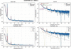
(i) Structural interpretation of the S1 fit. The mean coherent domain size of M_mean = 10 layers (∼123 Å) with a log-normal spread of σ_M = 2 layers is consistent with values reported for SWy-2 Na-montmorillonite in the 1W state by Drits & Tchoubar (1990) and Oueslati et al. (2012). The spacing disorder σ_d = 0.50 Å is physically reasonable: it accounts for the distribution of interlayer cation positions and local water configurations without introducing the Debye–Mering extinction of higher-order 00l reflections prematurely. The near-total extinction of the 002 reflection – reproduced without any adjustable parameter – constitutes an internal validation of the layer structure factor formulation (Bailey, 1988). Destructive interference between the two Si–O tetrahedral sheets is geometrically exact only for the correct TOT layer charge distribution, and its reproduction confirms the consistency of the layer structure factor throughout (Fig. 1).

Figure 1 Experimental and calculated scattering intensity for sample S1 (43% RH, oriented film, equilibrium 1W state). The total model (solid line) is decomposed into SAXS, basal 00l and hkl contributions. The 001 reflection (d001 ≃ 12.3 Å) is well reproduced in both position and intensity. This dataset provides the reference parameters for the fully hydrated 1W state with minimal disorder.

(ii) SAXS–XRD junction calibration. The junction coupling coefficient scale_00l = 0.115 was measured directly from the normalized experimental curve as the ratio I_exp(q₀₀₁)/I_max(SAXS). Its low value for S1 (0.115) reflects the dominance of the SAXS signal over the 001 reflection in a material with relatively large platelets (L₀ = 110 Å), consistent with the expectation that the Porod decay of large platelets is still significant at q₀₀₁ ≃ 0.51 Å⁻¹.

(iii) Goodness of fit. The domain-specific RMSE values (Table 4) confirm that the model provides a statistically adequate description in all three structural regimes. The slightly elevated residual in the junction zone (RMSE = 0.044, versus 0.028 in the SAXS domain and 0.031 in the 00l domain) reflects the intrinsic sensitivity of this region to multiple structural parameters, and this behaviour is further quantified in Section 5.3. Importantly, the residuals in the junction zone are spatially localized around the wing of the 001 reflection and do not indicate a systematic model deficiency.

Table 4
Structural parameters and goodness-of-fit metrics for sample S1 (oriented film, 43% RH, pure 1W reference state)

Parameters marked with a dagger directly address the SAXS–XRD junction. RMSE values were computed on normalized intensities over the indicated q domains. The 002 extinction is reproduced without adjustment (internal validation of DATFS).

Parameter	Value	Physical interpretation
d0(1W) (Å)	12.3	Mean 1W basal spacing; assigns the 001 position at q001 ≃ 0.511 Å^−1
σd (Å)	0.50	Gaussian width of interlayer spacing distribution; controls higher-order 00l extinction via the Debye–Mering factor
Tij	[[1.0]]	Single-state Markov matrix; by construction π = [1.0], enforcing pure 1W stacking; zero interstratification
Mmean, Mσ	10, 2	Log-normal coherent domain size: mean of 10 layers (∼123 Å) with moderate polydispersity
L0, σL (Å)	110, 55	Platelet lateral diameter distribution (Gaussian); controls Guinier knee position and SAXS slope
qjoin, Δq (Å^−1)	0.38, 0.03	Sigmoid crossover parameters; qjoin is set below q001 to ensure the 001 reflection is fully assigned to the 00l module
scale00l	0.115	Dimensionless coupling amplitude measured from normalized experimental curve: Iexp(q001)/Imax(SAXS)
wturb	0.052	Turbostratic hkl amplitude; linear regression over inter-peak domains (0.6–3.0 Å^−1)
RMSESAXS	0.028	RMSE in the SAXS domain (q < 0.38 Å^−1)
RMSEjunction	0.044	RMSE in the junction zone (0.38–0.60 Å^−1) including the 001 reflection
RMSE00l	0.031	RMSE over higher-order basal reflections (q > 0.60 Å^−1)

4.2. In-plane structure validation: sample S1 as disordered powder

The powder diffractogram of sample S1 provides the sole direct experimental window on the turbostratic hkl contribution. Because the Bragg–Brentano geometry of an oriented film selects only planes perpendicular to the scattering vector, i.e. the (00l) planes, the in-plane (hk) scattering is systematically suppressed in the film configuration and can only be measured in a geometrically isotropic (powder) setup.

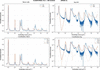
The Debye-based formulation reproduces both the position and the overall envelope of the turbostratic band centred at q ≃ 1.41 Å⁻¹ with RMSE = 0.026, a satisfactory level of agreement given the complexity of the in-plane correlations. The Warren asymmetry profile (abrupt low-q edge, exponential high-q tail) characteristic of two-dimensional turbostratic structures is correctly reproduced, confirming that the in-plane pair-correlation function computed from the Bailey atomic positions (Bailey, 1988) is physically representative of the Na-montmorillonite TOT layer.

Systematic discrepancies in the fine structure of the band, where the experimental signal exhibits sharper sub-band oscillations than the calculated Debye curve, are attributed to residual in-plane crystallographic order (finite two-dimensional coherence) that is not captured by the azimuthal-average approximation. This effect is expected in a first-order Debye treatment and does not affect the dominant band shape or position. Quantitatively, these deviations correspond to length scales below 5 Å (below the resolution limit relevant for clay mineral characterization) and do not propagate into the stacking analysis (Fig. 2).

Figure 2 Experimental and calculated scattering intensities in the turbostratic hkl domain for the disordered powder configuration (S1). (Top panels) Comparison between experimental data (solid lines) and calculated total intensity (dashed lines) on linear (left) and logarithmic (right) scales. The main turbostratic band centred around q ≃ 1.4 Å^−1 ( reflection) is reproduced in both position and overall envelope. (Bottom panels) Decomposition of the calculated intensity into basal 00l and turbostratic hkl contributions, shown in linear (left) and logarithmic (right) representations. The hkl component dominates the intermediate and high-q range, while the residual 00l contribution becomes negligible in the powder configuration. The Debye-based formulation (Poiarkova & Rehr, 1999; Gelisio & Scardi, 2016) captures the characteristic asymmetric profile of turbostratic scattering, although fine structural deviations remain visible in the logarithmic representation. These deviations are attributed to residual in-plane correlations and limitations of the isotropic Debye approximation. The overall agreement supports the use of a global in-plane disorder parameter (σr) and a fixed turbostratic weight (wturb) in subsequent analyses of oriented samples.

The powder calibration of w_turb = 0.15 and σ_r = 0.40 Å forms the basis of the parameter hierarchy and is transferred unchanged to all subsequent film analyses (S4, S2, S3). This locking prevents the turbostratic contribution from acting as an adjustable background in the higher-q domain during the stacking fits, which would otherwise introduce a systematic compensation error in the σ_d determination. The elevated RMSE in the 00l domain for the powder (0.069, versus 0.031 for the oriented film) is expected: a random powder orientation mixes the scattering contributions from all crystallographic planes, reducing the sensitivity to coherent basal stacking (Table 5).

Table 5
Parameters used for S1 powder simulation (turbostratic hkl calibration)

All stacking parameters are fixed from the S1 film analysis. The w_turb and σ_r values calibrated on this dataset are locked for all subsequent oriented-film fits. RMSE_hkl = 0.026 is the primary validation criterion.

Parameter	Value	Status/interpretation
d0(1W) (Å)	12.3	Fixed from S1 film; no re-optimization
σd (Å)	0.50	Fixed from S1 film
Tij	[[1.0]]	Fixed (pure 1W, no interstratification)
Mmean	10	Fixed from S1 film
wturb	0.15	Calibrated on powder; transfers to all subsequent film analyses
σr (Å)	0.40	Two-dimensional Debye–Waller factor; calibrated on powder dataset
RMSE (hkl domain)	0.026	Good agreement on band shape and position
RMSE (00l domain)	0.069	Expected: powder geometry reduces sensitivity to stacking coherence

4.3. Morphological decoupling: sample S4

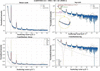
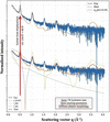
Sample S4 was prepared by differential sedimentation to reduce the mean platelet lateral dimension while preserving the same 1W hydration state and stacking characteristics observed in S1. The unchanged position of the 001 reflection confirms that the observed variation is predominantly morphological rather than crystallographic (Figs. 3 and 4).

Figure 3 Comparison of experimental and calculated scattering intensities for samples S1 and S4 (43% RH, identical hydration state, different particle sizes). While the basal reflections remain unchanged, significant differences are observed in the low-q region. The model reproduces these variations through changes in the platelet size distribution, confirming that morphological parameters primarily control the SAXS regime.

Figure 4 Direct comparison of samples S1 and S4 in the SAXS-dominated region. Both samples exhibit the same 1W hydration state and comparable stacking characteristics, while differing in platelet morphology. The reduction of the mean platelet lateral size from L0 = 110 Å (S1) to L0 = 60 Å (S4) shifts the Guinier knee from q ≃ 0.20 Å^−1 to q ≃ 0.35 Å^−1 while leaving the position of the basal 001 reflection essentially unchanged. The comparison demonstrates that the principal difference between S1 and S4 is morphological rather than crystallographic.

The reduced platelet size of S4 has a measurable effect on the scattering pattern. A diagnostic feature distinguishing S4 from S1 is the significant enhancement of the low-q scattered intensity, which is directly attributable to the increase in the specific surface area of smaller platelets and the corresponding shift of the Guinier knee to higher q values. Quantitatively, reducing L₀ from 110 Å (S1) to 60 Å (S4) shifts the position of the Guinier crossover from q ≃ 0.20 Å⁻¹ to q ≃ 0.35 Å⁻¹, compressing the SAXS regime and increasing the relative overlap with the 001 reflection. This compression is correctly reproduced by the model without any modification of the stacking parameters.

The junction coupling coefficient scale_00l increases substantially from 0.115 (S1) to 1.88 (S4). This large variation is not a fitting artefact but reflects a genuine physical difference: smaller platelets have a weaker SAXS form factor at q₀₀₁ (because the Porod decay for a disc of radius R scales as R⁻² at q ≫ 1/R), while the 001 reflection amplitude is controlled by stacking coherence M and is the same in S1 and S4. The ratio I_exp(q₀₀₁)/I_max(SAXS) therefore increases as the platelets become smaller, consistent with the Porod scaling argument. This behaviour validates the junction coupling scheme as physically self-consistent across different morphological regimes (Table 6).

Table 6
Structural parameters for sample S4 (fine fraction, 43% RH), with details of how they differ from the results for sample S1

The systematic increase in scale_00l from 0.115 (S1) to 1.88 (S4) is a direct physically interpretable consequence of the Porod decay scaling with platelet size, not a fitting parameter.

Parameter	Value	Comment or variation versus S1
d0(1W) (Å)	12.3	Unchanged; identical hydration state confirms same crystallographic structure
σd (Å)	0.70	Slight increase versus S1 (0.50 Å); consistent with higher surface/volume ratio in fine particles introducing marginally greater local spacing heterogeneity
Mmean, Mσ	9, 2	Comparable to S1; sedimentation does not alter stacking coherence
L0 (Å)	60	Reduced by ∼45% versus S1 (110 Å); primary morphological variable in S4
σL (Å)	50	Narrower distribution reflects size-selective sedimentation
scale00l	1.88	Higher than S1 (0.115): smaller platelets reduce SAXS intensity, increasing the relative weight of the 00l contribution at the junction
RMSESAXS	0.097	Higher sensitivity in SAXS domain, expected given the dominant role of morphology for S4
RMSEjunction	0.061	Improved versus S1; smaller platelets shift the Porod decay to higher q, reducing overlap at the junction
RMSE00l	0.035	Comparable to S1; stacking description is unaffected by size selection

The basal reflections of S4 are located at the same positions and exhibit RMSE_00l = 0.035, comparable to that of S1 (0.031), confirming that sedimentation-based size selection does not alter the stacking structure. The slight increase in σ_d (from 0.50 to 0.70 Å) may reflect an increased proportion of particle edges in the fine fraction, where interlayer forces are weaker and spacing fluctuations are larger, or alternatively a statistical effect of the smaller sample size. It does not indicate a fundamentally different stacking mechanism.

4.4. Markov description of equilibrium interstratification: sample S2

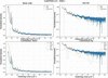
Sample S2, equilibrated at 54% RH for ≥5 days, represents the thermodynamic equilibrium of the 1W/2W interstratified state. Its scattering pattern cannot be reproduced by a simple linear combination of the S1 (pure 1W) and a hypothetical pure 2W pattern, because such an additive model – the classical I_classical(q) = ∑α w_α I_α(q) formulation (Drits & Tchoubar, 1990) – neglects the coherent cross terms between layers of different hydration states within the same stack. These cross terms produce the characteristic diffuse inter-peak background that is the experimental fingerprint of intra-stack heterogeneity (Fig. 5).

Figure 5 Experimental and calculated scattering intensities for sample S2 (54% RH, equilibrium conditions). The 1W–2W interstratification is described using a Markov-chain stacking model. The shape and asymmetry of the 001 region and the diffuse background between reflections are reproduced, indicating the presence of correlated intra-stack heterogeneity.

The transition matrix T = [[0.85, 0.15], [0.20, 0.80]] encodes the conditional probabilities of hydration state transitions between adjacent layers. The diagonal elements T₁₁ = 0.85 and T₂₂ = 0.80 indicate a strong self-persistence of each state: a given 1W layer has an 85% probability of being followed by another 1W layer, and a 2W layer has an 80% probability of being followed by another 2W layer. The off-diagonal elements T₁₂ = 0.15 and T₂₁ = 0.20 control the transition frequency and determine the mean run length of each state [mean 1W run: 1/(1 − T₁₁) = 6.7 layers; mean 2W run: 1/(1 − T₂₂) = 5 layers].

The stationary distribution π ≃ [T₂₁/(T₁₂ + T₂₁), T₁₂/(T₁₂ + T₂₁)] = [0.571, 0.429] predicts approximately 57% 1W and 43% 2W layers at equilibrium, a proportion consistent with the experimentally observed relative amplitudes of the 1W and 2W 001 reflections.

The inter-peak background that distinguishes S2 from a simple two-phase mixture arises from the interference between the structure factors of adjacent layers of different types. For a 1W–2W pair, the phase difference Δφ = q(d_2W − d_1W)/2 ≃ 1.5q Å is q dependent, producing a constructive or destructive interference pattern that is spread across the junction region rather than concentrated at the 00l peak positions. This diffuse background is the physical signature of short-range interstratification and cannot be reproduced by any additive model.

The experimental origin of these features can be inspected directly in Fig. S3, which shows the measured S1 and S2 profiles in the SAXS–XRD crossover region without model superposition or decomposition. In particular, the S2 profile clearly displays the 2W 001 and 1W 001 reflections, together with the diffuse inter-peak background associated with intra-stack heterogeneity.

Regarding higher-order 2W reflections, the 2W 004 reflection is consistently underestimated, suggesting that the current two-water-layer model for the 2W state does not fully account for all scattering contributions. Possible explanations include (i) the presence of a minor fraction of 3W layers (d_3W ≃ 18.5 Å) at 54% RH, which would contribute a weak reflection at q ≃ 0.34 Å⁻¹ overlapping with the 2W 001 wing; (ii) symmetry-breaking in the 2W interlayer due to Na⁺ off-centring, which would modify the interlayer structure factor; or (iii) orientation-dependent form factor effects not accounted for in the 1D stacking projection. These discrepancies are confined to specific reflections and do not affect the Markov matrix determination, which is constrained primarily by the shape and asymmetry of the 001 doublet region (Table 7).

Table 7
Structural parameters for sample S2 (equilibrium 1W/2W interstratification, 54% RH)

The Markov matrix is the only free parameter group for this dataset. The stationary distribution π ≃ [0.57, 0.43] derived from T_ij is consistent with the observed relative 001 amplitudes. The 2W 004 underestimation is discussed in Section 5.7.

Parameter	Value	Physical interpretation
d0(1W) (Å)	12.3	Fixed from S1 reference
σd(1W) (Å)	0.50	Fixed from S1 reference
d0(2W) (Å)	15.3	Characteristic 2W basal spacing; positions 2W 001 at q ≃ 0.411 Å^−1
σd(2W) (Å)	1.00	Larger than 1W; reflects less constrained interlayer water configuration in the 2W state
Tij	[[0.85, 0.15], [0.20, 0.80]]	Markov transition matrix at equilibrium; stationary distribution π ≃ [0.57, 0.43], giving ∼57% 1W and ∼43% 2W layers
Reichweite R	1	Short-range order (R = 1); only nearest-neighbour correlations considered, first-order Markov chain
Initial state distribution (π0)	None (stationary π)	Chain initialized at stationary distribution, thermodynamic equilibrium assumption fully satisfied
Mmean	10	Fixed from S1
L0 (Å)	110	Fixed from S1 morphology, identical sample origin
qjoin (Å^−1)	0.33	Shifted below S1 value to include the 2W 001 reflection (q ≃ 0.411 Å^−1) in the 00l domain
scale00l	0.786	Measured on the 001 window (0.35–0.60 Å^−1) encompassing both 1W and 2W 001 reflections
RMSE00l	0.033	Best performance over the basal domain, Markov description captures interstratification accurately

4.5. Non-equilibrium kinetics: sample S3

Sample S3 is measured under the same humidity target (54% RH) as S2 but with a deliberately short equilibration time (<2 h), capturing the system in a transient interstratified state that has not yet reached the thermodynamic equilibrium described by S2. The central hypothesis is that the short-range transition probabilities (matrix T) are thermodynamically determined and remain unchanged relative to S2, while the global abundance of each hydration state evolves kinetically and is therefore not described by the stationary distribution π.

The non-stationary initial state distribution π₀ = [0.93, 0.07] means that 93% of stacking sequences are initialized in the 1W state, reflecting the experimental condition: the sample was in a stable 1W state (43% RH, as S1) prior to the humidity jump to 54%, and only 1 h 45 min of exposure was allowed before acquisition. The initial state distribution therefore represents the macroscopic 1W/2W population ratio at the time of measurement, which is distinct from the local transition probability T₁₂ governing the sequence of states within a stack once a 2W domain has nucleated.

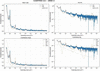
The increased spacing disorder of the 2W state [σ_d(2W) = 1.80 Å, versus 1.00 Å at equilibrium] reflects the structural heterogeneity of nascent 2W domains that have not yet organized their interlayer water molecules into the well defined two-layer configuration characteristic of equilibrium. The parameter σ_d(2W) is therefore interpretable as a kinetic disorder metric: its value is expected to decrease monotonically as the equilibration time increases, approaching the S2 value of 1.00 Å at full equilibrium (Fig. 6).

Figure 6 Experimental and calculated scattering intensity for sample S3 (54% RH, non-equilibrium conditions). Compared with the profiles for S2, deviations are observed in the junction region and in the width of basal reflections. These features are reproduced by introducing a non-stationary state distribution and increased spacing disorder, consistent with a kinetically evolving stacking structure.

The phase-noise term (σ_φ = 0.30) introduces stochastic fluctuations in the accumulated phase of each layer contribution, simulating the effect of local structural defects (edge dislocations, incomplete interlayer hydration or microstrain) that disrupt the coherent stacking. This term is physically distinct from σ_d: while σ_d represents the thermal and static width of the d-spacing distribution (a structural thermodynamic quantity), the phase-noise perturbation represents a dynamic or defect-driven coherence loss that is transient and would disappear at equilibrium. Its activation in S3 and deactivation in S2 is therefore physically motivated.

The junction region is sensitive to kinetic effects. The RMSE in the junction zone of S3 (0.112) is the highest across all the samples, reflecting the fact that the non-equilibrium condition produces the most complex intensity distribution in the region where multiple contributions overlap. The simultaneous presence of incomplete 2W domains (broad σ_d), kinetic phase disorder (the phase-noise perturbation) and a non-stationary state population (π₀) all contribute to the junction residuals. Importantly, however, the RMSE in the 00l domain remains identical to that for S2 (0.033), confirming that the local stacking mechanism is the same and that the increased junction residual is attributable to population and disorder effects rather than to a different structural mechanism (Table 8).

Table 8
Structural parameters for sample S3 (non-equilibrium interstratification, 54% RH, kinetic state)

Parameters differing from S2 indicate kinetic deviations. The identity of T_ij between S2 and S3 is a key result: short-range layer correlations are thermodynamically determined, while the global state population is kinetically controlled.

Parameter	Value	Interpretation or contrast with S2
d0(1W) (Å)	12.3	Unchanged
d0(2W) (Å)	15.3	Unchanged
σd(1W) (Å)	0.30	Slightly reduced versus S2; 1W layers remain well ordered at short equilibration
σd(2W) (Å)	1.80	Strongly increased versus S2 (1.00 Å): nascent 2W domains have incomplete water organization; broader spacing distribution
Tij	[[0.85, 0.15], [0.20, 0.80]]	Fixed from S2; local transition probabilities are thermodynamically determined, not kinetically altered
Initial state distribution (π0)	[0.93, 0.07]	Non-stationary initial distribution: 93% 1W at chain initialization, reflecting incomplete water uptake after 1 h 45 min of RH conditioning
Phase-noise perturbation	Enabled (σφ = 0.30)	Stochastic phase perturbation introduced to represent local structural defects and additional coherence loss during non-equilibrium hydration
Δq (Å^−1)	0.05	Broader junction transition width versus S2 (0.03); reflects increased uncertainty in the 001 region due to state redistribution
RMSEjunction	0.112	Highest residual across all samples; expected in the non-equilibrium state where population and spacing disorder are both maximal
RMSE00l	0.033	Identical to S2; same Tij, same local stacking mechanism

4.6. Cross-sample synthesis: multi-scale RMSE and parameter consistency

Table 9 consolidates the goodness-of-fit metrics across all datasets, providing a quantitative basis for assessing the internal consistency of the unified model. Several structural trends emerge from this comparison:

Table 9
Cross-sample RMSE summary for all experimental datasets, organized by q domain

RMSE values computed on normalized intensities. A dash (–) indicates that the domain is not applicable for the given measurement configuration. `Fixed' for S2 and S3 SAXS indicates that SAXS parameters were locked from S1/S4 and not re-fitted.

Sample	RMSESAXS	RMSEjunction	RMSE00l	RMSEhkl
S1 (film)	0.028	0.044	0.031	–
S1 (powder)	–	–	0.069	0.026
S4 (fine)	0.097	0.061	0.035	–
S2 (equilibrium)	Fixed	0.052	0.033	–
S3 (kinetic)	Fixed	0.112	0.033	–

(i) Domain-specific RMSE hierarchy. The junction zone consistently exhibits a relatively high RMSE across all samples, reflecting its intrinsic multi-parameter sensitivity. The 00l domain RMSE is systematically lower (0.031–0.035 for equilibrium samples), confirming that the Markov stacking model accurately describes the basal reflection profiles once the structural parameters are properly constrained. The turbo­stratic hkl domain shows the lowest RMSE (0.026 for S1 powder), consistent with the physical simplicity of the in-plane Debye formulation.

(ii) Morphological scaling of scale_00l. The junction coupling coefficient scale_00l varies from 0.115 (S1, large platelets) to 1.88 (S4, fine fraction), tracking the Porod decay of the platelet form factor as a function of L₀. This monotonic behaviour provides an independent validation of the junction coupling scheme, demonstrating that scale_00l is not a free fitting parameter but a physically constrained coupling observable.

(iii) Kinetic signature in RMSE_junction. The large RMSE in the junction zone for S3 (0.112) relative to S2 (0.052) provides a quantitative metric for deviation from equilibrium. This difference is consistent with a possible diagnostic role for RMSE_junction in future time-resolved studies, though this application remains to be validated (see Section 6.4).

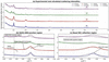
A global comparison of all datasets is shown in Fig. 7. This figure integrates experimental data and model predictions, and their decomposition into SAXS, 00l and hkl contributions across all samples. The simultaneous agreement across independent datasets confirms the internal consistency of the parameter-locking strategy. Residual and enlarged representations further highlight the sensitivity of the junction and 001 regions, providing a detailed assessment of model performance at critical structural scales.

Figure 7 Multi-sample comparison between experimental and calculated scattering intensities for samples S1–S4. Experimental data (solid lines) and calculated profiles (dashed lines) are shown using a common normalization and vertical offset for clarity. (a) Global comparison over the full scattering range, illustrating the overall agreement between experiment and model for all samples. (b) Enlargement of the SAXS–XRD junction region (q ≃ 0.30–0.70 Å^−1), highlighting the overlap between morphology-sensitive and stacking-sensitive scattering contributions. The positions of the 2W 001 and 1W 001 reflections and the diffuse inter-peak background are indicated. (c) Enlargement of the basal 001 reflection region (q ≃ 0.42–0.55 Å^−1), illustrating the sensitivity of the model to hydration state and interstratification. Detailed logarithmic representations, physical decompositions of the calculated intensity and residual analyses are provided in Figs. S4–S6.

5. Sensitivity analysis and parameter identifiability

The present section addresses the identifiability of the structural parameters of the unified model, the degree of coupling between parameters in different spectral domains, and the intrinsic limitations that constrain the precision and uniqueness of the inversion. The analysis draws on the stepwise experimental design of Section 3 and the fitting results of Section 4, and should be read in conjunction with the model limitations described in Section 5.7.

Parameter identifiability in disordered-system scattering is a fundamentally different problem from Rietveld refinement of crystalline phases: the observable plot is a continuous smooth function of q, not a set of discrete peak positions and integrated intensities, and the structural descriptors (M, T_ij, σ_d) are statistical moments of distributions rather than unique atomic coordinates. The approach adopted here – partitioning the q space into physically distinct domains, each sensitive to a different parameter subset, and using a nested experimental protocol to lock parameters sequentially – is the most effective strategy available in the absence of a fully automated inversion algorithm.

5.1. q-space domain decomposition and parameter sensitivity

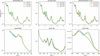
The central principle of the identifiability strategy is that the three structural contributions to the total intensity – SAXS morphology, 00l stacking and turbostratic hkl – have distinct and largely non-overlapping sensitivities in reciprocal space. This partitioning is not absolute – the junction region is precisely where the separation breaks down – but it provides a practical framework for parameter assignment that is quantitatively supported by the sensitivity maps of Fig. 8 (Section 5.8).

The SAXS domain (q < 0.38 Å⁻¹) is exclusively sensitive to the platelet form factor and therefore to the morphological parameters L₀, σ_L and t. At q < 1/(πL₀) (the Guinier regime) the intensity varies as , where R_g is the platelet gyration radius; the position of the Guinier knee directly encodes R_g and hence L₀. At q > 1/(πL₀) (the Porod regime) the intensity varies as q⁻² (infinite disc) or q⁻⁴ (finite disc with sharp boundary), encoding the polydispersity σ_L. The stacking parameters (M, d₀, σ_d, T) contribute negligibly to this domain, as demonstrated by the S1 versus S4 comparison: changing L₀ from 110 to 60 Å leaves the 001 position and width unchanged.

The 00l basal domain (0.40 < q < 2.5 Å⁻¹) carries information on stacking periodicity (d₀), disorder (σ_d), coherent domain size (M) and interstratification (T). The sensitivity of each parameter to the 00l profile is as follows: (i) d₀ determines the peak position with high precision (Δd ≃ 0.01 Å per 0.002° shift in 2θ for Cu Kα); (ii) σ_d controls the Debye–Mering decay of higher-order reflections [the 00l intensity scales as ], making σ_d well constrained by the relative intensities of successive 00l orders; (iii) M controls the peak width via the Debye–Scherrer relation [β ∝ 1/(Md₀)]; (iv) T controls the shape and asymmetry of the 001 doublet and the intensity of the inter-peak background.

The turbostratic hkl domain (q > 0.6 Å⁻¹) is controlled by the in-plane pair-correlation function, parameterized by the Debye weight w_turb and the two-dimensional Debye–Waller factor σ_r (Lele & Anantharaman, 1966; Gelisio & Scardi, 2016; Birmpilis et al., 2019a; Basak et al., 2022). These two parameters are independently calibrated on the S1 powder dataset and are insensitive to stacking parameters: the in-plane atomic positions of the TOT layer are the same for all hydration states (the interlayer water does not contribute to in-plane scattering) and the turbostratic hkl signal is therefore a mineral-specific constant that does not need to be re-optimized for S2 or S3.

5.2. The nested parameter-locking protocol and its role in identifiability

The experimental design explicitly exploits the domain decomposition described above to implement a sequential parameter-locking protocol. The nesting order is: S1 film (morphology + stacking baseline) → S1 powder (turbostratic calibration) → S4 (morphological perturbation) → S2 (Markov matrix, equilibrium) → S3 (kinetic deviation). At each stage, the parameters constrained in all preceding stages are fixed, and only the parameters associated with the new structural variable are adjusted.

This protocol has two key consequences for identifiability: (i) the effective dimensionality of each inversion is reduced from the full parameter space (∼14 parameters) to a small subset (typically 2–4 parameters per dataset), greatly reducing the risk of degeneracy; (ii) parameters determined at an early stage carry no uncertainty amplification from subsequent fits, because they are not re-adjusted. The main limitation of this approach is that it assumes the locked parameters are truly invariant between samples, which may not be strictly satisfied for natural clay materials with inherent batch-to-batch variability.

5.3. The junction region: source of maximum parameter coupling

The junction zone, defined here as 0.38 < q < 0.60 Å⁻¹ and containing the 001 reflection, is the region of maximum parameter coupling in the model. The intensity in this zone depends simultaneously on L₀ (Porod decay of the form factor), M (peak width), σ_d (Debye–Mering factor), T (shape of 001 doublet in interstratified systems) and scale_00l (relative amplitude coupling). This multi-parameter sensitivity is the physical reason why the junction RMSE is generally relatively high and it is the fundamental reason why an empirical hard boundary between SAXS and XRD is an inadequate treatment of this region.

The L₀–scale_00l coupling between the platelet lateral size L₀ and the junction amplitude scale_00l is the most important coupling in the junction zone. As L₀ increases, the Porod decay of the form factor shifts to lower q, increasing the form factor contribution at q₀₀₁ and therefore decreasing scale_00l = I_exp(q₀₀₁)/I_max(SAXS). The key mitigating factor is that scale_00l is not fitted – it is measured directly from the experimental curve – so this coupling does not introduce a free-parameter degeneracy. Instead, it means that the independently constrained value of L₀ (from the Guinier regime) and the independently measured value of scale_00l can be checked for self-consistency, providing an additional internal validation of the model.

A well known coupling in 00l analysis is the partial degeneracy between M (coherent domain size) and σ_d (spacing disorder). Both parameters contribute to peak broadening: M via the Debye–Scherrer term and σ_d via the Debye–Mering Gaussian damping (Benfatto et al., 1989). The two contributions have different functional forms – the Debye–Scherrer broadening is Lorentzian in 1/M (Lele & Anantharaman, 1966), while the Debye–Mering factor is Gaussian (Li et al., 2007) in lσ_d – but in practice, when only one or two 00l reflections are observed with a limited signal-to-noise ratio, the two effects can be partially conflated. In the present study, the simultaneous availability of at least three 00l orders (001, 003, 004 for S2) and the constraint from the junction SAXS regime (which independently constrains M via the platelet thickness t = Md₀₀₁) greatly reduces this degeneracy.

5.4. Identifiability of the Markov transition matrix

The Markov transition matrix T is the most structurally informative parameter group in the model and the most difficult to determine uniquely. For a two-state system (1W/2W), T has two independent parameters (T₁₂ and T₂₁, with T₁₁ = 1 − T₁₂ and T₂₂ = 1 − T₂₁). These parameters independently control (i) the stationary distribution π = [T₂₁/(T₁₂ + T₂₁), T₁₂/(T₁₂ + T₂₁)], which sets the long-range 1W/2W abundance; (ii) the mean run length of each state 〈n_α〉 = 1/(1 − T_αα), which controls the degree of short-range order; and (iii) the amplitude of the cross-term interference, which generates the inter-peak background.

The sensitivity analysis of Fig. 8 (variation of T₁₂) demonstrates that a change of ±0.05 in T₁₂ produces a measurable modification of the 001 region profile, specifically in the relative amplitudes of the 1W and 2W 001 components and in the breadth of the inter-peak background. This sensitivity is sufficient to constrain T₁₂ to within ±0.05 for samples with a well resolved 001 doublet (S2). However, for samples with strong spectral overlap (S3), the precision degrades because the non-stationary state distribution π₀ and the increased σ_d(2W) produce similar broadening effects.

T_ij and π₀ are coupled. In the non-equilibrium analysis of S3, the Markov matrix T and the initial state distribution π₀ [p₁, 1 − p₁] are not orthogonal: both affect the relative amplitudes of the 1W and 2W 001 contributions. The key physically motivated constraint that breaks this degeneracy is that T is fixed from S2: if the short-range thermodynamic interactions that govern nearest-neighbour state transitions are the same for S2 and S3 (which is a physically justified assumption, since the interactions depend on interlayer chemistry, not on the global hydration level), then π₀ is the only free parameter controlling the state abundance difference between S2 and S3. This reduces the S3 inversion to a single-parameter determination (Méring, 1949; Drits & Tchoubar, 1990; Plançon, 2002).

5.5. Sensitivity to morphological parameters

The sensitivity of the SAXS regime to platelet morphology (L₀, σ_L) is high but exhibits the characteristic behaviour of disc form factors: the Guinier region (q < 1/R_g) is sensitive to the mean platelet size, while the Porod slope (q > 1/R_g) is sensitive to the width of the size distribution. This means that for monodisperse samples L₀ and σ_L can be independently determined from the two q regimes. For polydisperse samples (σ_L/L₀ > 0.5, as for S1 and S4), the Guinier regime is smoothed and the knee position provides an effective radius that conflates the two parameters (Guinier et al., 1955).

Cross-sample comparisons can be decoupled from the stacking. The S1 versus S4 comparison confirms that L₀ changes from 110 to 60 Å with no measurable effect on the 00l RMSE (0.031 versus 0.035), demonstrating that morphological and stacking parameters can be treated as functionally independent to a first approximation. The residual coupling through scale_00l (which increases from 0.115 to 1.88) is quantitatively accounted for by the Porod scaling argument and does not introduce a fitting degeneracy.

5.6. Non-equilibrium indicators: distinguishing kinetic from structural disorder

The analysis of S3 introduces two kinetic parameters, the initial state distribution (π₀) and phase-noise perturbation, that are absent from the equilibrium description. Their identifiability rests on the distinction between their spectral signatures (Ferrage et al., 2005):

(i) Initial state distribution π₀ (population deviation). A non-stationary initial distribution π₀ modifies the relative amplitudes of the 1W and 2W 001 reflections without significantly broadening individual peaks. Its effect is primarily in the intensity ratio of the 001 doublet components and is therefore distinguishable from that of σ_d (which broadens individual peaks) and from changes in T (which modify both the ratio and the inter-peak background).

(ii) Phase-noise perturbation (coherence loss). The phase-noise term produces a diffuse continuous reduction in coherent scattering amplitude across the entire 00l domain, analogous to a Debye–Waller factor but for structural defects rather than thermal vibrations. Its spectral signature is a q²-dependent amplitude reduction that cannot be reproduced by σ_d (which has an l²q² dependence, i.e. it affects higher orders more strongly). This functional difference provides a basis for separating the two parameters, although in practice the degeneracy increases when only the 001 reflection is resolved.

The distinct spectral signatures of the non-stationary initial-state distribution (π₀) and the phase-noise perturbation were further investigated through a dedicated sensitivity analysis (Section S5: Fig. S7 and Table S3). The results show that π₀ primarily affects the relative amplitudes of the 1W 001 and 2W 001 reflections, whereas the phase-noise perturbation produces a broader redistribution of intensity across the junction region. Their combined action is required to reproduce the experimental S3 profile.

At this point we have to make a caveat. The distinction between a non-stationary initial distribution π₀ and a modified T matrix is subtle when the 001 doublet is poorly resolved, as in strongly disordered or small-M systems. The present study benefits from the sequential parameter-locking strategy in which T is constrained from S2, which eliminates this ambiguity. In the absence of an equilibrium reference dataset, the two effects would be degenerate and the distinction between equilibrium interstratification and kinetic non-equilibrium could not be made from the diffraction data alone.

5.7. Model limitations: quantitative assessment

The following limitations have been identified in the present model, ordered by their impact on the quantitative accuracy of the structural parameters (Besson & Drits, 1997):

(i) Systematic underestimation of higher-order 2W reflections. The 2W 004 reflection (and, to a lesser extent, 2W 002) is consistently underestimated in S2 and S3. Three distinct mechanisms could account for this discrepancy, with different implications for the model.

(a) An incomplete 2W structure factor. The current two-water-layer model assigns fixed atomic positions (z_Ow1 = 1.55 Å, z_Ow2 = 2.65 Å) and fixed occupancies (occ_Ow1 = 0.8, occ_Ow2 = 1.2) that may not represent the actual interlayer water structure at 54% RH. A more detailed model (e.g. MD simulation-derived positions) could improve the 2W structure factor at higher q.

(b) Presence of a 3W minority. A small fraction (<5%) of three-water-layer domains (d_3W ≃ 18–19 Å) would contribute an intensity near the 2W 004 position and its omission from the model would result in a systematic underestimation.

(c) Na⁺ off-centring and layer charge heterogeneity. The DATFS formulation treats all octahedral sites as equivalent (uniform Al/Mg substitution), while real montmorillonite has a heterogeneous charge distribution that perturbs the interlayer cation positions and modifies the structure factor at higher q.

(ii) Debye formulation smoothing of the hkl domain. The azimuthal average implicit in the Debye equation suppresses the angular dependence of the in-plane structure factor, producing a smoothed approximation to the turbostratic band. This is adequate for the band (the dominant feature in the accessible q range) but would fail for systems with significant in-plane crystalline order (e.g. low-defect chlorite or muscovite) where the hk0 reflections are resolved. For Na-montmorillonite, the turbostratic disorder is strong enough that the Debye approximation is physically justified.

(iii) First-order Markov (Reichweite R = 1) approximation. The R = 1 Markov chain assumes that the hydration state of layer k depends only on the state of layer k − 1, not on earlier layers. This approximation is exact for independently nucleated domains but may underestimate the correlation length in systems with cooperative hydration transitions (e.g. smectites with strong layer-charge heterogeneity). Extending to R = 2 (Besson & Drits, 1997) would add 2 × 2 = 4 additional transition parameters and would require datasets with more resolved higher-order reflections for constraint.

(iv) Sigmoid junction as an approximation. The sigmoid weighting function w(q) enforces a smooth but mathematically arbitrary crossover between the SAXS and 00l contributions. While the crossover position q₀ and width Δq are physically motivated (q₀ < q₀₀₁, Δq ≪ q₀₀₁), the sigmoid functional form does not derive from a rigorous diffraction theory.

The sigmoid weighting function should not be interpreted as implying that the SAXS contribution physically vanishes above q₀ or that the 00l contribution is absent below q₀. Rather, it provides a computational partition of the intensity aimed at avoiding double counting in a region where morphology and stacking information overlap. The resulting intensity therefore represents a phenomenological crossover approximation rather than a rigorous decomposition of the scattering cross section.

A physically exact treatment would require computing the full three-dimensional scattering function of a polydisperse stack ensemble, which is computationally intractable for disordered systems of realistic size. The sigmoid approximation is therefore a pragmatic solution whose validity is supported by the low junction RMSE for S1 and S4 (0.044 and 0.061), but it may break down for systems with very strong morphological disorder or for q₀₀₁ values close to the SAXS boundary.

The validation of the junction reported in Section 6.6.2 relies on an internally consistent hierarchy of samples measured on the same instrument (S1, S4) rather than on an independent external dataset, for example synchrotron SAXS combined with laboratory XRD acquired on the same physical sample. The low RMSE_junction values obtained for S1 and S4 therefore demonstrate the internal consistency and computational adequacy of the sigmoid approximation under the tested conditions, but do not constitute an independent exper­imental validation of the junction coupling. Such a cross-instrument validation is identified as a priority for future work (Section 6.9).

The sensitivity of the SAXS–XRD crossover parameters was evaluated through a dedicated analysis of q₀ and Δq. Variations in q₀ of ±0.02 Å⁻¹ and in Δq of ±0.01 Å⁻¹ produced only moderate changes in the junction-region RMSE and did not alter the principal structural conclusions. Detailed results are provided in Table S4 and Fig. S8.

5.8. Summary of parameter identifiability

A detailed identifiability analysis is provided in Tables S5 and S6. Table S5 provides a qualitative correlation matrix for the main model parameters, summarizing the pairwise coupling identified in Sections 5.3–5.6. `High' indicates that the two parameters produce nearly indistinguishable spectral effects in the relevant domain, `moderate' indicates partial coupling that is broken by the experimental design and `low' indicates negligible coupling (Fig. 8).

Figure 8 Sensitivity of the calculated scattering intensity to selected model parameters, evaluated around the S2 equilibrium configuration. (Top row) Full q range. (Bottom row) Corresponding enlargements of characteristic regions. (Left-hand column) Variation of platelet size (L0), primarily affecting the SAXS regime. (Middle column) Variation of interlayer spacing disorder (σd), controlling peak broadening in basal reflections. (Right-hand column) Variation of the Markov transition probability (T12), modifying the shape of the 001 region. The localized response of the intensity demonstrates limited parameter degeneracy.

The overall conclusion of the identifiability analysis is that the unified model is over-determined (more experimental constraints than free parameters) when the full five-dataset protocol is applied, and that the main parameter degeneracies are effectively broken by the combination of domain decomposition, direct measurement of scale_00l, sequential parameter locking and the S2 → S3 transfer of T. The primary remaining source of uncertainty is the M–σ_d coupling in the 00l domain, which could be reduced by independent determination of M from atomic force microscopy measurements of platelet thickness, or by exploiting the SAXS constraint on t = Md₀₀₁.

6. Discussion, broader implications and limitations

The results of Sections 4 and 5 collectively demonstrate that the unified CLADIFFMOD formalism provides a physically consistent and numerically tractable description of X-ray scattering from disordered Na-montmorillonite across a q range spanning more than one decade (0.14–4.5 Å⁻¹). This section discusses the broader significance of this result in the context of the clay mineral characterization literature, examines the implications of the key physical findings, and provides a frank assessment of the limitations that must be acknowledged before the model can be applied in routine analytical contexts.

6.1. The SAXS–XRD separation

The present work proposes a computationally tractable approximation for addressing the SAXS–XRD crossover. This aim is achieved by constructing a single intensity function that contains both contributions simultaneously. The key insight is that the apparent incompatibility between the two approximations is not a fundamental physical obstacle: it reflects the absence, until now, of a computationally accessible formalism that combines a realistic platelet form factor with a stochastic stacking model and a junction coupling condition. The sigmoid junction is not a phenomenological patch – its crossover parameters are physically determined (q₀ < q₀₀₁, Δq → 0) and the coupling amplitude scale_00l is directly measurable from experimental data.

The most concrete demonstration of this internal consistency is the self-consistency of the coherent domain size M across the two domains. In the unified framework, M simultaneously controls the width of the 001 reflection (via the Debye–Scherrer term in the 00l module) and the platelet thickness t = Md₀₀₁ (via the SAXS form factor). For S1, the fitted M = 10 layers implies t ≃ 123 Å, consistent with the form factor input parameter. This self-consistency would be impossible to verify in a classical independent analysis, because the two determinations of M would use different datasets, different instruments and different fitting routines without any mutual constraint. This consistency check is internal to the present dataset series and does not by itself constitute an external validation of the junction coupling against an independent measurement [Section 5.7(iv)]

6.2. Intra-stack heterogeneity as a physical mechanism

The Markov-chain description of intra-stack hydration sequences was introduced by Drits & Tchoubar (1990) as a formal mathematical framework, and its equivalence to the matrix formalism was demonstrated by Plançon (2002). What the present work adds is the direct visualization of the physical consequence of intra-stack heterogeneity in the scattering pattern – specifically, the diffuse inter-peak background between the 1W and 2W 001 reflections in sample S2 – and the demonstration that this feature cannot be reproduced by any additive population model, regardless of the number of components or the sophistication of the fitting algorithm.

The physical origin of the inter-peak background is the coherent interference between the structure factors of adjacent layers of different types within the same stack. For a 1W–2W pair at layer positions z_k and z_k+1, the cross-term contribution to the intensity is 2Re{(q)F_2W(q)exp[iq(z_k+1 − z_k)]}. This term oscillates in q at a frequency determined by the mixed spacing (d_1W + d_2W)/2 ≃ 13.8 Å, producing a broad diffuse background centred between the 1W and 2W 001 positions. An additive model, which computes the intensity of each layer type independently and sums the results, explicitly discards these cross terms and therefore cannot reproduce this background.

T_ij has a thermodynamic interpretation. The fitted Markov matrix T = [[0.85, 0.15], [0.20, 0.80]] determined from S2 is consistent with a picture in which both 1W and 2W states are locally stable at 54% RH, with a per-junction transition probability of ∼15–20%. We stress, however, that, as discussed in Section 6.6.3, T is not uniquely determined by the diffraction data alone, so the specific numerical values T₁₁ = 0.85 and T₂₂ = 0.80, and any quantitative thermodynamic reading of their difference (e.g. in terms of relative activation energies), should be regarded as model-dependent rather than as directly measured quantities. What is robustly established by the data, independent of this degeneracy, is (i) the existence of intra-stack heterogeneity itself, i.e. the 1W and 2W layers coexist within individual stacks rather than as separate populations, and (ii) the diffuse inter-peak background as its diffraction fingerprint, which cannot be reproduced by any additive model regardless of the exact T values used to generate it.

The present analysis is directly consistent with the conclusions of our previous work (Odom, 1984; Oueslati et al., 2012; Oueslati et al., 2015; Oueslati & Meftah, 2018), where we demonstrated, using the Drits matrix formalism, that the quantitative analysis of smectite hydration sequences at intermediate RH requires the explicit treatment of 1W/2W coexistence within a single coherent domain. The present work extends this conclusion to the SAXS regime by demonstrating that the same intra-stack heterogeneity that shapes the 00l profile also affects the SAXS contribution through the coherent domain size M and the junction coupling coefficient scale_00l.

6.3. Decoupling morphology from crystallography: implications for clay characterization

The S1 versus S4 comparison – same hydration state, different platelet size – provides the first direct experimental demonstration, within a single self-consistent analysis framework, that morphological and stacking parameters can be independently constrained from the X-ray scattering pattern of a clay suspension or film. This has some practical implications:

(i) Reinterpretation of peak broadening in conventional XRD. In conventional XRD-only analysis of clay minerals, peak broadening is typically attributed to a combination of small M, large σ_d and interstratification. The present results demonstrate that the SAXS contribution from small platelets also broadens the effective 001 peak at the junction – a contribution that is entirely absent from XRD-only models (Oueslati, 2026b). This means that XRD-derived values of M from fine-grained clay samples may be systematically underestimated if the SAXS contribution at the junction is misattributed to peak broadening rather than to form factor overlap. Quantitatively, the effect is significant for L₀ < 80 Å and becomes negligible for L₀ > 200 Å.

(ii) Implications for colloidal and rheological studies. The platelet lateral dimensions L₀ and σ_L determined from the SAXS regime of the same diffraction pattern that provides stacking parameters represent a significant analytical advantage for studies of clay suspensions, gels and nanocomposites, where both morphology (controlling rheology and aggregation) and stacking (controlling swelling and ion exchange) are simultaneously relevant. The present framework provides these parameters from a single measurement rather than requiring separate SAXS and XRD acquisitions (Birmpilis et al., 2019a).

6.4. RMSE_junction as a candidate state indicator

A practical, but as yet untested, outcome of the junction analysis is that RMSE_junction (the root-mean-square residual in the crossover region) differs markedly between the three states examined here: 0.044 (S1, single-state equilibrium), 0.052 (S2, two-state equilibrium) and 0.112 (S3, kinetic non-equilibrium). We stress that these are three discrete independently equilibrated (or deliberately non-equilibrated) samples, rather than sequential snapshots of a single relaxation process. The observed ordering is therefore consistent with, but does not by itself establish, a general relationship between RMSE_junction and the degree of thermodynamic disequilibrium (Ferrage et al., 2007).

We propose RMSE_junction as a candidate diagnostic for time-resolved in situ hydration studies, but this application should be regarded as a hypothesis rather than a validated capability. At least three points remain open: (i) whether RMSE_junction increases monotonically with disequilibrium along a genuine kinetic trajectory (a single humidity-jump experiment sampled at several time points, rather than three distinct equilibrated states, would be required to test this); (ii) the sensitivity of RMSE_junction to counting statistics and measurement noise, which has not been characterized and could set a detection floor below which kinetic changes are not resolvable; and (iii) whether the absolute RMSE_junction scale reported here (0.044–0.112) is specific to the SWy-2 reference smectite or would generalize, in some rescaled form, to other 2:1 clay mineralogies with different layer spacings and Markov transition statistics.

Establishing RMSE_junction as a quantitative kinetic index will require a dedicated time-resolved dataset, a noise-propagation/reproducibility analysis and a cross-mineralogy comparison, none of which fall within the scope of the present three-sample equilibrium/non-equilibrium study (Chipera & Bish, 2001).

6.5. Comparison with classical approaches

Table 10 summarizes the key differences between the present unified formalism and the classical independent SAXS/XRD approach. The comparison is organized by the physical aspects of the clay mineral scattering problem, allowing a structured assessment of where the unification provides the most significant advances.

Table 10
Structured comparison of the present unified SAXS–XRD formalism with the classical independent approach for disordered clay mineral characterization

Criterion	Classical independent approach	Present unified formalism
Treatment of 001 reflection	Assigned to XRD only; SAXS contribution at q001 ignored	Simultaneously constrained by SAXS form factor and 00l stacking model
Coherent domain size M	Determined independently from SAXS (Guinier) and XRD (Debye–Scherrer); no mutual constraint (Guinier et al., 1955)	Single unified determination from joint fit; Md001 = t constrains both SAXS and 00l domains
Interstratification model	Additive populations (homogeneous stacks), I = ∑wαIα (Drits & Tchoubar, 1990; Plançon, 2002) – incorrect†	Markov intra-stack heterogeneity; cross-terms reproduced, diffuse inter-peak background quantitatively described
Turbostratic scattering	Treated as unstructured background or ignored	Debye equation (Bailey, 1988); calibrated independently on powder dataset, locked for all film analyses
Kinetic or non-equilibrium states	Not addressable within stationary Markov formalism	A non-stationary initial state distribution π0 separates population kinetics from the local stacking mechanism
Parameter consistency	No mutual constraint between SAXS and XRD parameters	All parameters determined from a single joint dataset, scale00l provides direct measurable coupling
Applicability	Domain-specific software (NEWMOD, AB2F, SAXS-specific programs) (Moore & Reynolds, 1997; Plançon, 2002)	Single CLADIFFMOD program, generalizable to any 2:1 clay through adaptation of the hydration-state definitions and Markov transition matrix

†The `incorrect' label for additive population models refers specifically to the treatment of intra-stack heterogeneity. these models are not incorrect in all contexts, but they are physically wrong for systems where layers of different types coexist within a single coherent domain.

6.6. Limitations revisited

The limitations identified in Section 5.7 deserve a more detailed physical discussion in the context of the broader clay mineral characterization literature, particularly for the purpose of establishing what the model does not claim to achieve.

6.6.1. The 2W structure factor uncertainty

The underestimation of the 2W 004 reflection, consistently observed across S2 and S3, is the most significant quantitative limitation of the current model. Its origin is almost certainly in the simplified treatment of the 2W interlayer structure: the current code assigns two water oxygen positions (z_Ow1 = 1.55 Å, z_Ow2 = 2.65 Å from the layer midplane) with occupancies 0.8 and 1.2 that were determined by trial and error from the S2 fit rather than from a crystallographically determined structure. The actual distribution of interlayer water molecules in an Na-smectite at 54% RH is a complex three-dimensional network whose projection onto the stacking axis has been modelled by molecular dynamics simulations (Meleshyn & Bunnenberg, 2006; Holmboe & Bourg, 2014) but has never been directly refined from X-ray data for the specific SWy-2 sample studied here.

The practical consequence of this limitation is that the 2W structure factor is systematically in error at high q. Specifically, the 004 and higher-order 2W reflections are not correctly predicted, while the 001 region, which determines the Markov matrix, is adequately described.

A dedicated sensitivity analysis of the 2W interlayer structure was performed (Table S7 and Fig. S9). Water-oxygen positions and occupancies were varied within physically reasonable limits, and the Markov parameters were re-optimized for each perturbed configuration. Although the amplitude of the 2W 004 reflection was measurably affected by these perturbations, the fitted transition probabilities T₁₂ and T₂₁ remained unchanged within the resolution of the optimization procedure. These results indicate that the principal conclusions regarding intra-stack heterogeneity and the inferred Markov matrix are robust with respect to moderate uncertainty in the 2W interlayer water structure.

6.6.2. The sigmoid junction as a physical approximation

The sigmoid weighting function does not derive from a rigorous scattering theory. Its use rests on the following physical argument: In the transition zone (0.35 < q < 0.60 Å⁻¹), the form factor and the stacking contributions cannot simply be added because they describe the scattering from the same physical entity (the clay stack) at the same length scale (the platelet thickness). The physically exact formulation would require computing |F_stack(q)P_disc(q_||, L)|² [where P_disc(q_||, L) denotes the platelet disc form factor and q_|| is the component of the scattering vector parallel to the platelet plane], averaged over all orientations – an integral that is analytically intractable for a polydisperse disordered stack ensemble. The sigmoid is therefore a computational compromise that preserves continuity of the intensity and its derivative across the junction, while distributing the two contributions in a q-dependent manner that is physically motivated by the crossover from morphology-dominated (q < q₀) to stacking-dominated (q > q₀) scattering.

A first assessment of the sigmoid approach is provided by its performance on S1, where the form factor parameters (from S4) and the stacking parameters (from S1 itself) are locked from other parts of the same dataset series, so that their combination at the junction is a genuine prediction rather than a free fit within that series. The resulting RMSE_junction = 0.044 for S1, obtained without any free parameter specific to the junction, indicates that the sigmoid approximation performs well under the tested conditions (Debye, 1915; Pedersen, 1997). We emphasize, however, that the data for S1 and S4 were acquired on the same instrument and the same reference material, and this internal cross check does not constitute an independent external validation, for example, against synchrotron SAXS combined with laboratory XRD on the same physical sample [Section 5.7(iv)]. The sigmoid junction should therefore be regarded as a computationally tractable approximation that performs well under the tested conditions, rather than as a definitively validated solution to the SAXS–XRD crossover problem. (Debye, 1915; Porod, 1982; Pedersen, 1997).

6.6.3. Uniqueness of the Markov inversion

The Markov transition matrix T is not uniquely determined by the diffraction data alone. For a given 001 profile, there may exist multiple combinations of [T₁₂, T₂₁, σ_d(2W), M] that produce equally good fits within experimental uncertainty. The degeneracy is reduced by the sequential locking protocol [M fixed from S1, σ_d(1W) fixed, σ_d(2W) constrained by the S3 comparison], but it cannot be entirely eliminated without additional experimental constraints, specifically, a second 00l order for the 2W state that is resolved from the 1W contribution.

In practice, the fitted T values should be interpreted as a representative Markov description of the stacking sequence – one that reproduces the observed diffraction pattern and whose stationary distribution is consistent with the observed 1W/2W abundance ratio – rather than as a unique determination of the nearest-neighbour transition probabilities. The physical interpretation in terms of thermodynamic stability and nucleation probability (Section 6.2) is contingent on this caveat. This distinction between robust conclusions (intra-stack heterogeneity and diffuse inter-peak scattering) and model-dependent interpretations (specific T values and their thermodynamic meaning) is discussed further in Section 6.2.

6.7. Extension to other 2:1 clay systems

The unified CLADIFFMOD formalism is, by construction, applicable to any 2:1 disordered clay mineral, not only Na-montmorillonite. The mineral-specific components are confined to two elements: the hydration-state definitions and the layer structure factor description [which uses the layer structure factor formalism of Bailey (1988) for the specific octahedral and tetrahedral composition]. Everything else – the Markov chain engine, the SAXS form factor, the Debye turbostratic module and the sigmoid junction – is mineral independent.

The most direct extensions are as follows:

(i) Ca-montmorillonite. The 2W state structure is significantly different from Na-montmorillonite (two water layers with Ca²⁺ centred between them versus off-centre Na⁺), requiring modified z_Ow and occupancy values in the 2W hydration-state definition.

(ii) Mixed-layer illite–smectite (IS). Requires adding an illite layer type (d₀ ≃ 10.0 Å, σ_d ≃ 0, fixed non-expandable layer) to the hydration-state definitions and extending the Markov matrix to 3 × 3 (or larger for R = 2 systems).

(iii) Vermiculite. Requires extending to R = 2 Markov chains to reproduce the strong short-range ordering characteristic of high-charge 2:1 minerals (Table 11).

Table 11
Extension roadmap for the CLADIFFMOD formalism: target systems, scientific motivation and required model additions

Note that all extensions maintain the same Markov + sigmoid junction + Debye architecture. Only the hydration-state definitions, the Markov matrix dimension and (for R = 2) the transition tensor need to be modified. TEM = transmission electron microscopy. SANS = small-angle neutron scattering.

Extension	Scientific motivation	Required additions
Mixed-layer illite–smectite (IS)	Most abundant clay mineral in diagenetic sequences; XRD complexity is the primary obstacle to quantitative IS characterization	Hydration-state definitions: add an illite layer type (d0 ≃ 10.0 Å, σd ≃ 0), Markov matrix extended to 3 × 3 (illite, 1W, 2W)
Vermiculite and high-charge smectites	Strong layer charge produces R = 2 ordering (Reichweite); additive models systematically underestimate correlation length	Extend Markov to R = 2 (next nearest neighbour); requires 2^2 × nstates transition tensor
Time-resolved in situ humidity cycling	Track hydration kinetics in real time; RMSEjunction provides quantitative non-equilibrium index	Time-parameterize the non-stationary initial state distribution π0(t) and σd(2W)(t); kinetic model for water uptake rate
Complementary techniques (NMR, TEM, SANS)	Independent constraint on M, L0 and interlayer water structure; reduce M–σd degeneracy	AFM platelet statistics → fix L0, σL; ^2H NMR → constrain water layer occupancies; SANS → validate form factor
Automated Bayesian inversion	Replace sequential locking with rigorous uncertainty quantification; compute posterior distributions for all parameters	Markov chain Monte Carlo (MCMC) sampler with physically motivated priors; computationally intensive but now feasible

6.8. Methodological implications for the clay mineralogy community

The present work has practical methodological implications beyond the specific results obtained for Na-montmorillonite. The most important are as follows:

(i) Reconsidering the knife-edge setting as a critical experimental parameter. The combination of SAXS and XRD in a single oriented-film experiment requires careful control of the knife-edge (couteau) position (Section 3.3.1). A misset of 0.1 mm produces a d₀₀₁ shift of ∼0.05 Å and a systematic error in q₀₀₁ that propagates directly into scale_00l. This is a measurement artefact that would be invisible in a conventional XRD-only analysis (where d₀₀₁ is calibrated against an Si standard) but becomes critical when scale_00l is used as a structural coupling parameter.

(ii) The 24 h acquisition time as a structural choice. The extended counting time (10 s per step below 2θ = 10°) is not merely a signal-to-noise improvement; it is essential for resolving the Guinier knee in the SAXS regime and for obtaining a statistically reliable estimate of the inter-peak background that distinguishes intra-stack interstratification from additive phase mixtures. This requirement should be explicitly stated in experimental protocols for joint SAXS–XRD clay mineral studies (Birmpilis et al., 2019b).

(iii) The powder configuration as an independent turbostratic calibration. The conventional practice of using only oriented films for clay mineral characterization by XRD systematically misses the turbostratic hkl contribution, which is suppressed in the Bragg–Brentano geometry of an oriented film. The present protocol – an oriented film for SAXS + 00l, a disordered powder for hkl – requires two measurements on the same sample but provides an unambiguous separation of the in-plane and out-of-plane scattering contributions that is not achievable from a single configuration.

6.9. Concluding perspective: towards a unified clay characterization standard

The SAXS–XRD junction problem, as defined in Sections 1 and 2 of this article, has been described for decades as an unsolved limitation of clay mineral characterization.

The present work demonstrates that the problem is computationally tractable – not by circumventing the physical complexity of the junction zone but by constructing a formalism that is explicitly designed to handle it and that performs well under the tested conditions. A definitive claim of resolution would require independent external validation [Section 5.7(iv)]; the present results should be read as an initial computationally tractable approximation rather than a full closure of the problem

The CLADIFFMOD implementation is not a definitive software tool; it will require further validation on a broader range of clay minerals, hydration states and experimental configurations before it can be proposed as a community standard. Nevertheless, the physical framework it embodies (the explicit coupling of SAXS morphology, Markovian intra-stack stacking and Debye turbostratic scattering through a physically motivated junction condition) represents a conceptual advance that is independent of the specific implementation details. Any future unified clay mineral scattering program will need to address the same three physical contributions and the same junction coupling problem.

The most important practical message of this work is that the coherent domain size M should never be determined from SAXS and XRD independently without checking for mutual consistency, and that such a check is only possible within a unified formalism of the type presented here. The systematic discrepancy between SAXS-derived and XRD-derived M values that has been noted (but not resolved) in the clay mineral literature is not a measurement artefact or a sample heterogeneity effect: it is a model deficiency that the present framework substantially reduces under the tested conditions, pending independent external validation.

7. Conclusions

This study presents a unified multi-scale approach for the interpretation of X-ray scattering from disordered 2:1 clay minerals, in which the SAXS, basal 00l and turbostratic hkl contributions are treated within a single continuous formalism. The results obtained from the five experimental datasets show that this combined description provides a consistent representation of the scattering signal over a broad q range, while maintaining a direct physical interpretation of all model parameters.

A central outcome of the work is the explicit treatment of the transition region between the small-angle and wide-angle domains. The analysis indicates that the 001 reflection, located at this junction, is influenced by both platelet morphology and stacking periodicity. By incorporating these effects simultaneously, the present framework reduces the inconsistencies that typically arise when SAXS and XRD are analysed independently.

The stepwise experimental design plays an important role in supporting this interpretation. The reference sample (S1) establishes the baseline structural parameters and validates the continuity of the SAXS–XRD coupling. The powder dataset confirms that the turbostratic hkl contribution can be constrained independently, while the fine fraction (S4) demonstrates that morphological parameters primarily affect the low-q region. These independent constraints provide a basis for interpreting the more complex interstratified and non-equilibrium systems.

The interstratified sample (S2) shows that a Markov-chain representation of the stacking sequence provides a plausible description of intra-stack heterogeneity. The resulting diffraction patterns suggest that short-range correlations between adjacent layers play a significant role in shaping the basal reflection profiles. At the same time, the analysis indicates that the corresponding parameters are not strictly unique and should be interpreted with some caution.

The kinetic dataset (S3) further suggests that deviations from equilibrium conditions may be detectable within the same framework. The introduction of a non-stationary state distribution and increased spacing disorder leads to modifications that are consistent with the observed diffraction patterns. While this interpretation appears physically reasonable, it remains dependent on modelling assumptions and would benefit from further validation.

Despite the overall consistency of the results, several limitations remain. In particular, the systematic underestimation of higher-order reflections indicates that the current description does not fully account for all aspects of stacking coherence. In addition, the Debye-based formulation of the turbostratic contribution provides an averaged representation that does not reproduce fine structural variations. These limitations suggest that the model should be regarded as an approximate description of a complex disordered system.

Within these constraints, the unified formulation offers a structured way to analyse multi-scale scattering data, in which different structural parameters are associated with distinct regions of reciprocal space. This approach may be useful for a range of disordered layered materials, particularly in cases where morphology, stacking structure and hydration state are closely coupled.

Overall, the results suggest that combining SAXS and XRD within a single framework can improve the internal coherence of structural interpretations, while also highlighting the complexity and limitations inherent in disordered clay systems. Further developments, including the integration of complementary experimental techniques and the extension of the model to more complex layer sequences, may help to refine and generalize the present methodology.

8. Supplementary materials

Supplementary materials accompanying this article are available online. They include (i) a description of the Monte Carlo implementation and computational workflow (Figs. S1 and S2); (ii) details of the humidity conditioning and instrumental parameters (Tables S1 and S2); (iii) logarithmic experimental versus calculated comparisons and decomposition analyses (Figs. S3–S6); (iv) sensitivity of the S3 junction region to the initial-state distribution (π₀) and the phase-noise perturbation (Fig. S7 and Table S3); (v) sensitivity of the SAXS–XRD junction parameters (q₀, Δq) for sample S1 (Fig. S8 and Table S4); (vi) parameter identifiability and correlation analyses (Tables S5 and S6); (vii) sensitivity analysis of the fitted Markov matrix and of the 2W 004 residual to the assumed 2W interlayer water structure (Table S7 and Fig. S9) and (viii) a glossary of symbols, parameters and abbreviations.

References

Ahn, J. H. & Buseck, P. R. (1990). Am. Mineral. 75, 267–275.
CAS
Google Scholar
Ammar, M., Oueslati, W., Ben Rhaiem, H. & Ben Haj Amara, A. (2014). J. Environ. Chem. Eng. 2, 1604–1611.
CrossRef
Anovitz, L. M. & Weston, J. (2020). Crystallization via Nonclassical Pathways, Vol. 1, Nucleation, Assembly, Observation & Application, pp. 201–257. American Chemical Society.
Anton Paar (2020). TTK 600 Low-Temperature Chamber: Instruction Manual. Anton Paar GmbH, Graz, Austria. https://www.anton-paar.com/corp-en/products/details/low-temperature-chamber-ttk-600/.
Bailey, S. W. (1969). Clays Clay Miner. 17, 355–371.
Web of Science
Bailey, S. W. (1980). Crystal Structures of Clay Minerals and Their X-ray Identification, edited by G. W. Brindley & G. Brown, ch. 1, pp. 1–123. London: Mineralogical Society.
Bailey, S. W. (1988). Clays Clay Miner. 36, 193–213.
Basak, M., Rahman, M. L., Ahmed, M. F., Biswas, B. & Sharmin, N. (2022). J. Alloys Compd. 895, 162694.
Beaucage, G. (1995). J. Appl. Cryst. 28, 717–728.
IUCr Journals
Benfatto, M., Natoli, C. R. & Filipponi, A. (1989). Phys. Rev. B 40, 9626–9635.
Besson, G. & Drits, V. A. (1997). Clays Clay Miner. 45, 158–169.
Besson, G., Mifsud, A., Tchoubar, C. & Mering, J. (1974). Clays Clay Miner. 22, 379–384.
Birmpilis, G., Ahmadi-Naghadeh, R. & Dijkstra, J. (2019a). Géotech. Lett. 9, 355–360.
Birmpilis, G., Hall, S. A., Lages, S. & Dijkstra, J. (2019b). Acta Geotech. 14, 1965–1975.
Bookin, A. S., Drits, V. A., Plançon, A. & Tchoubar, C. (1989). Clays Clay Miner. 37, 297–307.
Brigatti, M. F. & Mottana, A. (2011). Editors. Layered Mineral Structures and their Application in Advanced Technologies. London: Mineralogical Society.
Brindley, G. W. (1980). Bull. Miner. 103, 395–403.
Britto, S., Joseph, S. & Vishnu Kamath, P. (2010). J. Chem. Sci. 122, 751–756.
Chaaya, R., Gaboreau, S., Milet, F., Maubec, N., Tremosa, J., Raimbourg, H. & Ferrage, E. (2023). Appl. Clay Sci. 245, 107124.
Chipera, S. J. & Bish, D. L. (2001). Clays Clay Miner. 49, 398–409.
Classen, S., Hura, G. L., Holton, J. M., Rambo, R. P., Rodic, I., McGuire, P. J., Dyer, K., Hammel, M., Meigs, G., Frankel, K. A. & Tainer, J. A. (2013). J. Appl. Cryst. 46, 1–13.
Dabat, T., Porion, P., Hubert, F., Paineau, E., Dazas, B., Grégoire, B., Tertre, E., Delville, A. & Ferrage, E. (2020). Appl. Clay Sci. 184, 105354.
Debye, P. (1915). Ann. Phys. 351, 809–823.
Drits, V. A. (1997). Modular Aspects of Minerals, edited by S. Merlino, ch. 2.4, pp. 153–192. Budapest: European Mineralogical Union.
Drits, V. A. (2003). Clay Miner. 38, 403–432.
Drits, V. A., Sakharov, B. A., Lindgreen, H. & Salyn, A. (1997). Clay Miner. 32, 351–371.
Drits, V. A., Sakharov, B. A., Salyn, A. L. & Manceau, A. J. C. M. (1993). Clay Miner. 28, 185–207.
Drits, V. A. & Tchoubar, C. (1990). X-ray Diffraction by Disordered Lamellar Structures: Theory and Applications to Microdivided Silicates and Carbons, pp. 233–303. Berlin, Heidelberg: Springer.
Feng, J., Kriechbaum, M. & Liu, L. (2019). Nanotechnol. Rev. 8, 352–369.
Ferrage, E., Lanson, B., Sakharov, B. A. & Drits, V. A. (2005). Am. Mineral. 90, 1358–1374.
Ferrage, E. (2016). Clays Clay Miner. 64, 348–373.
Ferrage, E., Lanson, B., Sakharov, B. A., Geoffroy, N., Jacquot, E. & Drits, V. A. (2007). Am. Mineral. 92, 1731–1743.
Frewein, M. P. K., Rumetshofer, M. & Pabst, G. (2019). J. Appl. Cryst. 52, 403–414.
Gelisio, L. & Scardi, P. (2016). Acta Cryst. A72, 608–620.
Giannini, C., Ladisa, M., Altamura, D., Siliqi, D., Sibillano, T. & De Caro, L. (2016). Crystals 6, 87.
Gilbert, B., Comolli, L. R., Tinnacher, R. M., Kunz, M. & Banfield, J. F. (2015). Clays Clay Miner. 63, 432–442.
Guggenheim, S. (2011). Layered Mineral Structures and their Application in Advanced Technologies, edited by M. F. Brigatti & A. Mottana, ch. 2, An Overview of Order/Disorder in Hydrous Phyllosilicates, pp. 73–121. London: Mineralogical Society.
Guinier, A., Fournet, G., Walker, C. B. & Yudowitch, K. L. (1955). Small-Angle Scattering of X-rays. New York: Wiley.
Guyonnet, D., Gaucher, E., Gaboriau, H., Pons, C. H., Clinard, C., Norotte, V. & Didier, G. (2005). J. Geotech. Geoenviron. Eng. 131, 740–749.
Hamley, I. W. (2022). Soft Matter 18, 711–721.
PubMed
Hammouda, B. (2010). J. Appl. Cryst. 43, 716–719.
Heftberger, P., Kollmitzer, B., Heberle, F. A., Pan, J., Rappolt, M., Amenitsch, H., Kučerka, N., Katsaras, J. & Pabst, G. (2014). J. Appl. Cryst. 47, 173–180.
Holmboe, M. & Bourg, I. C. (2014). J. Phys. Chem. C 118, 1001–1013.
Hu, N., Borkar, N., Kohls, D. & Schaefer, D. W. (2011). J. Membr. Sci. 379, 138–145.
Jensen, H., Pedersen, J. H., Jørgensen, J. E., Pedersen, J. S., Joensen, K. D., Iversen, S. B. & Søgaard, E. G. (2006). J. Exp. Nanosci. 1, 355–373.
Johnston, C. T. (2010). Clay Miner. 45, 245–279.
Kaler, E. W. (1988). J. Appl. Cryst. 21, 729–736.
Kline, S. R. (2006). J. Appl. Cryst. 39, 895–900.
Kloprogge, J. T., Komarneni, S. & Amonette, J. E. (1999). Clays Clay Miner. 47, 529–554.
Lanson, B. (2005). Clay Sci. 12(Suppl. 1), 1–5.
Lanson, B. (2011). Layered Mineral Structures and their Application in Advanced Technologies, edited by M. F. Brigatti & A. Mottana, ch. 4, pp. 151–202. London: Mineralogical Society.
Lanson, B. & Besson, G. (1992). Clays Clay Miner. 40, 40–52.
Lanson, B., Sakharov, B. A., Claret, F. & Drits, V. A. (2009). Am. J. Sci. 309, 476–516.
Lele, S. & Anantharaman, T. R. (1966). Proc. Indian Acad. Sci. Sect. A 64, 261–274.
Leu, L., Georgiadis, A., Blunt, M. J., Busch, A., Bertier, P., Schweinar, K., Liebi, M., Menzel, A. & Ott, H. (2016). Energy Fuels 30, 10282–10297.
Li, R., Han, X. E., Shi, L., Ren, K. F. & Jiang, H. (2007). Appl. Opt. 46, 4804–4812.
Loganathan, N., Ferguson, B. O., Arey, B., Argersinger, H. E. & Bowers, G. M. (2020). J. Phys. Chem. A 124, 9832–9843.
Malwitz, M. M. (2005). PhD thesis, Louisiana State University and Agricultural and Mechanical College, Baton Rouge, Louisiana, USA.
Marangoni, A. G. & Pensini, E. (2026). Cryst. Growth Des. 26, 2369–2378.
Mejri, C., Oueslati, W. & Amara, A. B. H. (2021). Adsorpt. Sci. Technol. 2021, 9732092.
Mejri, C., Oueslati, W. & Ben Haj Amara, A. (2023a). Appl. Surf. Sci. Adv. 15, 100403.
Mejri, C., Oueslati, W. & Ben Haj Amara, A. (2023b). Clays Clay Miner. 71, 513–538.
Meleshyn, A. & Bunnenberg, C. (2006). J. Phys. Chem. B 110, 2271–2277.
Méring, J. (1949). Acta Cryst. 2, 371–377.
Mermut, A. R. & Cano, A. F. (2001). Clays Clay Miner. 49, 381–386.
Moll, W. F. Jr (2001). Clays Clay Miner. 49, 374–380.
Moore, D. M. & Reynolds, R. C. (1997). X-ray Diffraction and the Identification and Analysis of Clay Minerals. Oxford University Press.
Morodome, S. & Kawamura, K. (2009). Clays Clay Miner. 57, 150–160.
Odom, I. E. (1984). Philos. Trans. R. Soc. London Ser. A 311, 391–409.
Oueslati, W. (2026a). Artif. Intell. Chem. 4, 100120.
Oueslati, W. (2026b). Particuology 110, 75–95.
Oueslati, W., Ammar, M. & Chorfi, N. (2015). Minerals 5, 507–526.
Oueslati, W., Ben Rhaiem, H. & Ben Haj Amara, A. (2012). Appl. Surf. Sci. 261, 396–404.
Oueslati, W., Benrhaiem, H., Lanson, B. & Benhajamara, A. (2009). Appl. Clay Sci. 43, 224–227.
Oueslati, W. & Meftah, M. (2018). Mater. Sci. Eng. 2018, 5219624.
Oueslati, W. & Meftah, M. (2026). Hybrid. Adv. 13, 100635.
Oueslati, W., Mejri, C. & Amara, A. B. H. (2022). Nanoclay – Recent Advances, New Perspectives and Applications, edited by W. Oueslati, ch. 1. London: IntechOpen.
Pabst, F. & Blochowicz, T. (2022). J. Chem. Phys. 157, 244501.
Pabst, W., Gregorová, E. & Tichá, G. (2007). J. Eur. Ceram. Soc. 27, 479–482.
Pedersen, J. S. (1997). Adv. Colloid Interface Sci. 70, 171–210.
Plançon, A. (2001). Clay Miner. 36, 1–14.
Plançon, A. (2002). Am. Mineral. 87, 1672–1677.
Plançon, A. & Drits, V. A. (2000). Clays Clay Miner. 48, 57–62.
Plançon, A. & Tchoubar, C. (1977). Clays Clay Miner. 25, 430–435.
Plançon, A. & Zacharie, C. (1990). Clay Miner. 25, 249–260.
Poiarkova, A. V. & Rehr, J. J. (1999). Phys. Rev. B 59, 948–957.
Pons, C. H. (1980). Evidence of Relationships Between Texture and Structure in Smectite Systems by Small-Angle Synchrotron X-ray Scattering. Report No. FRCEA-TH-8295. Universite d'Orleans, UER de Sciences Fondamentales et Appliquées, France.
Porod, G. (1982). Small-Angle X-ray Scattering, edited by O. Glatter & O. Kratky. Academic Press.
Ramsay, J. D. F. & Lindner, P. (1993). Faraday Trans. 89, 4207–4214.
Reynolds, R. C. Jr (1985). NEWMOD. A Computer Program for the Calculation of One-dimensional Diffraction Patterns of Mixed-layered Clay. Hanover, New Hampshire, USA.
Reynolds, R. C. Jr (1993). Computer Applications to X-ray Powder Diffraction Analysis of Clay Minerals, edited by R. C. Reynolds Jr & J. R. Walker, ch. 3, pp. 43–78. Boulder: Clay Minerals Society.
Sakharov, B. A. & Drits, V. A. (1973). Clays Clay Miner. 21, 15–17.
Sakharov, B. A. & Drits, V. A. (2015). Lithol. Miner. Resources 50, 50–79.
Sakharov, B. A., Drits, V. A., McCarty, D. K. & Walker, G. M. (2016). Clays Clay Miner. 64, 314–333.
Sakharov, B. A., Plançon, A., Lanson, B. & Drits, V. A. (2004). Clays Clay Miner. 52, 680–692.
Sato, T., Watanabe, T. & Otsuka, R. (1992). Clays Clay Miner. 40, 103–113.
Shang, C., Rice, J. A., Eberl, D. D. & Lin, J. S. (2003). Clays Clay Miner. 51, 293–300.
Singh, P. S. (2017). Membrane Characterization, edited by N. Hilal, A. F. Ismail, T. Matsuura & D. Oatley-Radcliffe, ch. 6, pp. 95–111. Amsterdam: Elsevier.
Środoń, J. (1999). Annu. Rev. Earth Planet. Sci. 27, 19–53.
Tchoubar, D. & Cohaut, N. (2006). Dev. Clay Sci. 1, 879–907.
Tuck, J. J., Hall, P. L., Hayes, M. H., Ross, D. K. & Poinsignon, C. (1984). J. Chem. Soc. Faraday Trans. 1 80, 309–324.
Vainio, U. (2014). Small-Angle X-ray Scattering. Singapore: Pan Stanford Publishing Pte Ltd.
Vali, H. & Köster, H. M. (1986). Clay Miner. 21, 827–859.
Waasmaier, D. & Kirfel, A. (1995). Acta Cryst. A51, 416–431.
Warren, B. E. (1941). Phys. Rev. 59, 693–698.
Warren, B. E. & Averbach, B. L. (1953). The Diffuse Scattering of X-rays, in Modern Research Techniques in Physical Metallurgy, pp. 95–130. American Society for Metals.
This is an open-access article distributed under the terms of the Creative Commons Attribution (CC-BY) Licence, which permits unrestricted use, distribution, and reproduction in any medium, provided the original authors and source are cited.