Theoretical explanation of spatial coherence and source size characterization by X-ray grating interferometry

Lu, Y.; Wang, Z.; Du, X.; Wang, Q.; Hu, L.

doi:10.1107/S1600577526010544

research papers

JOURNAL OF
SYNCHROTRON
RADIATION

ISSN: 1600-5775

Volume 34| Part 1| January 2027|

https://doi.org/10.1107/S1600577526010544

Open

access

Theoretical explanation of spatial coherence and source size characterization by X-ray grating interferometry

Yujie Lu,^a Zimeng Wang,^a Xuewei Du,^a Qiuping Wang ^a and Lingfei Hu ^a ^*

^aNational Synchrotron Radiation Laboratory, University of Science and Technology of China, Hefei, Anhui 230029, People's Republic of China
^*Correspondence e-mail: [email protected]

Edited by H. Tolentino, Brazilian Synchrotron Light Laboratory, Brazil (Received 6 May 2026; accepted 13 October 2026)

The unprecedented spatial coherence of modern diffraction-limited storage rings (DLSRs) enables advanced X-ray experimental techniques. A precise beam characterization will be very helpful to exploit these techniques. Although X-ray grating interferometry (XGI) is widely used for this purpose, our previous work showed that the XGI-measured visibility width is significantly smaller than the coherence length (defined by the width of the local complex coherence function) for highly coherent beams [Lu et al. (2025), Opt. Lett. 50, 6746–6749]. To clarify what XGI actually probes, we present here a theoretical analysis. We show that, under the assumption of a global quadratic phase profile for the incident beam, XGI measures the normalized integrated cross-spectral density (ICSD), which represents a global correlation function of the beam. Based on this, we derive an analytical formula for exact coherence length measurement for ideal Gaussian Schell-model beams. Despite this difference from the coherence length, XGI yields reliable source size estimates. To explain this interesting fact, we use the ICSD to show that XGI can measure the source size within an acceptable error, even for DLSRs, provided the cross-spectral density of the source satisfies the Schell-model condition in mean and difference coordinates.

Keywords: spatial coherence; source size; X-ray grating interferometry; diffraction-limited storage ring.

1. Introduction

The advent of diffraction-limited storage rings (DLSRs) represents a significant advance in X-ray science. By delivering beams with extremely low emittance and high spatial coherence, these sources enable coherence-demanding techniques such as coherent diffraction imaging (Chushkin & Zontone, 2025 ), X-ray photon correlation spectroscopy (Narayanan et al., 2025 ), and ptychography (Pfeiffer, 2017 ). To fully exploit the potential of DLSRs, precise characterization of spatial coherence and source size is indispensable, as these parameters directly reflect the underlying electron beam emittance and guide beamline optimization (Trebushinin et al., 2024 ; Shi et al., 2025 ; Samadi et al., 2020 ).

Several approaches have been developed to characterize beam parameters. Young's double-slit method is the textbook standard, but its scanning nature makes it inefficient for multi-directional or routine diagnostics (Leitenberger et al., 2001 ; Takayama et al., 1998 ). Coded apertures such as uniform redundant arrays (URAs) (Nugent & Trebes, 1992 ; Lin et al., 2003 ) and non-redundant arrays (NRAs) (Skopintsev et al., 2014 ; Duarte et al., 2021 ), as well as speckle-based methods like heterodyne near-field speckle (HNFS) (Alaimo et al., 2014 ; Bagschik et al., 2016 ; Siano et al., 2022 ), have been proposed to overcome these limitations. In parallel, X-ray grating interferometry (XGI) has emerged as a practical and widely adopted technique, largely due to the availability of high-quality commercial gratings and its compatibility with existing beamlines (Bagschik et al., 2020 ; Marathe et al., 2014 ; Pfeiffer et al., 2005 ). Recently, theoretical studies have investigated how these grating structures affect the spatial coherence of highly coherent beams (Khubbutdinov et al., 2024 ; Vartanyants, 2024 ).

There are several metrics for the spatial coherence of synchrotron radiation (SR) beams, such as the global degree of coherence (Bei et al., 2010 ; Vartanyants & Singer, 2020 ), coherence area (Goodman, 2015 ; Vartanyants & Singer, 2020), and coherent flux (Khubbutdinov et al., 2019 ; Geloni et al., 2015 ). Apart from these metrics, the spatial coherence of the SR beam is normally described by the coherence length. It can be defined by the width of the modulus of the local complex coherence function (CCF), which is the normalized cross-spectral density (CSD) (Goodman, 2015). Previous works often interpret the visibility curve measured by XGI as the modulus of the local CCF (Pfeiffer et al., 2005; Marathe et al., 2014; Qi et al., 2014 ; Zhang et al., 2023 ). Thus, the coherence length of the beam can be derived by the width of the visibility curve. However, our recent study (Lu et al., 2025 ) shows that, when applied to DLSRs, the visibility width inferred from XGI becomes more than 30% smaller than the CCF width obtained from reference measurements such as Young's double-slit method. Interestingly, XGI remains a valuable tool for source size characterization [see equation (19) in this paper] (Shi et al., 2025; Zhang et al., 2023; Li, 2025 ) despite this difference between the measured width of the visibility curve and the width of the local CCF. This raises a fundamental question: why do the source sizes inferred from the same interferograms remain reliable while the widths of the visibility curves appear unexpectedly small? To answer this, it is essential to explain exactly what physical quantity XGI measures. In this paper, we revisit the physics of XGI. We show that XGI measures the normalized integrated cross-spectral density (ICSD) if the phase of the beam can be approximated by a quadratic polynomial. We will define ICSD later in this paper. The ICSD represents a global CSD over the entire beam. It differs from the local CCF. This deviation will be apparent when the beam size is small, or the CCF is not shift-invariant.

The remainder of this article is as follows. In Section 2, we focus on the general theory of XGI. We derive the ICSD and use it to find a simple analytical correction for the ideal Gaussian Schell-model (GSM) beam (Friberg & Sudol, 1982 ; Coïsson & Marchesini, 1997 ) and the real SR beam. The analytical correction is validated by numerical simulation. In Section 3, we discuss the XGI for source size measurement based on the ICSD. We find that, if the source CSD satisfies the Schell-model condition in mean and difference coordinates, XGI can yield a reliable source size measurement. We establish a link between the measured visibility curve and the source size. We reveal the physical limitation of XGI in a deeply diffraction-limited region. Section 4 summarizes this work.

2. General theory of XGI

2.1. XGI under general conditions

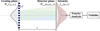
We begin by describing the basic physics model of XGI as shown in Fig. 1. The grating is illuminated by an X-ray beam with arbitrary spatial coherence. For simplicity, we restrict the analysis to a single transverse coordinate x. Let W_in(x₁, x₂) denote the CSD of the incident beam at positions x₁ and x₂. The one-dimensional periodic grating is described by its transmission function T(x). For a grating with period d, T(x) can be expressed as a Fourier series (Munro et al., 2010 ; Tang et al., 2023 ),

$[T\left(x\right) = \sum\limits_n {{c_n}\exp\left({i2\pi nx/d}\right)}, \eqno(1)]$

where c_n is the nth Fourier coefficient of the grating. Immediately after the grating, the CSD is modulated as (Goodman, 2015)

$[\eqalignno{ W^{\,\prime}({x_1},{x_2}) & = {W_{\rm{in}}}({x_1},{x_2})\,{T^{\,*}}({x_1})\,T({x_2}) & (2) \cr& = \sum\limits_{m,n} c_m^*c_nW_{\rm{in}}(x_1,x_2) \exp\left[{{i2\pi}\over{d}}\left(nx_2-mx_1\right)\right]. }]$

The modulated field then propagates a distance z to the detector plane. Under the paraxial approximation, this propagation is described by the Fresnel diffraction integral. The CSD at the observation plane, W_out(u₁, u₂, z), is given by (Goodman, 2015; Vartanyants, 2024; Khubbutdinov et al., 2024)

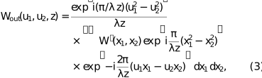
$[\eqalignno{ W_{\rm{out}}(u_1,u_2,z) = {}& {{\exp\big[i(\pi/\lambda{z})(u_1^2-u_2^2)\big]}\over{\lambda{z}}} \cr& \times \int\!\!\!\int W^{\,\prime}(x_1,x_2) \exp\left[i{{\pi}\over{\lambda{z}}}(x_1^2-x_2^2)\right] \cr& \times \exp\left[-i{{2\pi}\over{\lambda{z}}}(u_1x_1-u_2x_2)\right] \,{\rm{d}}x_1\,{\rm{d}}x_2, & (3) }]$

where λ is the wavelength and u is the coordinate on the detector plane. The intensity at the detector is obtained from the CSD, I_out(u, z) = W_out(u, u, z). Substituting equation (2) into equation (3) yields the general expression for the diffracted intensity,

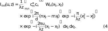
$[\eqalignno{ I_{\rm{out}}(u,z) = {}& {{1}\over{\lambda{z}}} \sum\limits_{m,n}c_m^{*}\,c_n \int\!\!\!\int W_{\rm{in}}(x_1,x_2) \cr& \times \exp\left[i{{2\pi}\over{d}}(nx_2-mx_1)\right] \exp\left[-i{{\pi}\over{\lambda{z}}}(x_1^2-x_2^2)\right] \cr& \times \exp\left[-i{{2\pi{u}}\over{\lambda{z}}}(x_1-x_2)\right] \,{\rm{d}}x_1\,{\rm{d}}x_2. & (4) }]$

To extract the information of spatial coherence, it is convenient to analyze the recorded intensity in the spatial-frequency domain (Cloetens et al., 1997 ; Guigay et al., 2004 ). The Fourier transform of I_out(u, z) with respect to u is Ĩ_out(f_u, z) = ∫I_out(u, z)exp(−i2πf_uu)du. By substituting the expression of I_out(u, z) and applying the scaling property of the Dirac delta function, we obtain

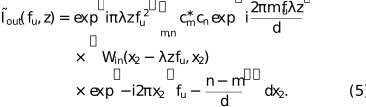
$[\eqalignno{ \tilde{I\,}\!_{\rm{out}}(\,f_u,z) = {}& \exp \left(i\pi\lambda{z}\,f_u^{\,2}\right) \sum\limits_{m,n}c_m^{*}\,c_n \exp \left(i{{2\pi{m}f_u\lambda{z}}\over{d}}\right) \cr& \times \int\! W_{\rm{in}}(x_2-\lambda{z}\,f_u,x_2) \cr& \times \exp\left[-i2\pi{x_2}\left(f_u-{{n-m}\over{d}}\right)\right]\,{\rm{d}}x_2. & (5) }]$

In XGI setups, the recorded pattern is dominated by interference between diffraction orders separated by a specific order difference n − m = p, where n, m and p are all integers. For example, the interference patterns of binary-amplitude and π/2 phase gratings are formed by neighboring diffraction orders (p = 1), while π phase gratings are dominated by the +1st and −1st orders (p = 2) (Pfeiffer et al., 2005; Marathe et al., 2014). The fringe visibility V(z) is thus proportional to the ratio of the first-order and zeroth-order Fourier components of the diffracted intensity, given by V(z) = |2Ĩ₁/Ĩ₀| (Pfeiffer et al., 2005; Marathe et al., 2014; Yashiro et al., 2018 ; Takeda et al., 1982 ). To derive an analytical expression for the visibility, we therefore evaluate equation (5) at these two spatial frequencies.

Figure 1
Schematic layout of XGI and the physics model for beam characterization. A partially coherent X-ray beam illuminates a grating with period d. After free-space propagation over a distance z, the interference between the diffraction orders produces a modulated intensity pattern I_out(u, z) at the detector plane. The fringe visibility is obtained from Fourier analysis.

For the zeroth-order, f_u = 0, only terms with n = m contribute. Other terms vanish during the integration due to the oscillatory phase. Therefore, the corresponding Fourier transform equals the total incident power weighted by the sum of the diffraction efficiencies of all orders,

$[\tilde{I\,}\!_0(0,z) \simeq \left(\sum\limits_m \left|c_m\right|^2\right) \int I_{\rm{in}}(x)\,{\rm{d}}x, \eqno(6)]$

where I_in(x) = W_in(x, x) is the incident intensity distribution. The first-order harmonic carries the information of interference, which originates from the diffraction orders with n = m + p. Assuming that the incident light field possesses a global quadratic phase profile with a radius of curvature R along x, the wavefront divergence causes a geometric magnification of the interference pattern. This results in a modified fringe period, given by d′ = d(1+z/R)/p. Consequently, the first-order harmonic is located at the modified spatial frequency, f_u = 1/d′. Specifically, for an ideal plane wave (R → ∞), the magnified period reduces to d′ = d/p, and this harmonic is simply located at f_u = p/d. By substituting f_u = 1/d′ and n = m + p into equation (5), the complex phase of the CSD and that related to the grating within the integral cancel each other out. This removes the rapid oscillations and leaves the modulus of the CSD. The corresponding Fourier transform can be written as

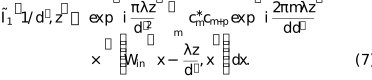
$[\eqalignno{ \tilde{I\,}\!_1\left(1/d^{\,\prime},z\right) \simeq {}& \exp\left(i\,{{\pi\lambda{z}}\over{d^{\,\prime2}}}\right) \sum\limits_m c_m^*c_{m+p} \exp\left(i\,{{2\pi{m}\lambda{z}}\over{dd^{\,\prime}}}\right) \cr& \times \int \left| W_{\rm{in}}\left(x-{{\lambda{z}}\over{d^{\,\prime}}},x\right) \right| \,{\rm{d}}x. & (7) }]$

The integral term in equation (7) is of central importance. It represents a line integral of the CSD modulus over the whole beam cross-section for a fixed transverse separation Δx = λz/d′. We now define this quantity as the integrated cross-spectral density (ICSD),

$[G\left(\Delta{x}\right) = \int \big| W_{\rm{in}} \left(x-\Delta{x},x\right) \big| \,{\rm{d}}x. \eqno(8)]$

G(Δx) is a global correlation across the entire beam cross-section. Fig. 2 elaborates on the meaning of the ICSD. The value of the ICSD at a specific Δx is equal to a line integration across the two-dimensional CSD modulus [Fig. 2(a)] along the diagonal path defined by x₂ = x₁ + Δx. The red line in Figs. 2(a) and 2(b) represents the special case when Δx = 0 µm. The CSD along this line is the intensity profile. Fig. 2(b) shows the normalized CSD modulus profiles for different Δx. Fig. 2(c) shows the normalized ICSD. It can be obtained by integrating the CSD modulus profiles shown in Fig. 2(b) over different values of Δx. The ICSD represents the global coherence property of the beam. It is different from the conventional local CCF, which only evaluates the correlation between a specific pair of points (Goodman, 2015).

Figure 2
(a) The modulus of a two-dimensional CSD. The dashed lines represent the integration paths for different Δx in equation (8)

. (b) The normalized CSD modulus along the respective dashed lines in (a). (c) The resulting modulus of the normalized ICSD curve |G(Δx)/G(0)|. G(Δx) is obtained by integrating the CSD profiles shown in (b).

As discussed above, the fringe visibility is proportional to the ratio of the first-order harmonic amplitude to the zeroth-order, V(z) = |2Ĩ₁/Ĩ₀|. Substituting equations (6)–(8) into the definition of fringe visibility, we have

$[V(z) \simeq \left| C_z {{G\left(\Delta{x}\right)}\over{G\left(0\right)}} \right|, \qquad \Delta{x} = {{\lambda{z}}\over{d^{\,\prime}}}, \eqno(9)]$

where C_z = $[2\exp(i\pi\lambda z/d^{\,\prime\,2}) \textstyle\sum_mc_m^{*}c_{m\,+\,p} \exp[i2\pi m\lambda z /(dd^{\,\prime})]]$ / $[\textstyle\sum_m |c_m|^2]$ is a factor that depends on the Fourier coefficient and the Talbot distance. Equation (9) shows that XGI probes the normalized ICSD.

To validate the theory proposed above, we also compare the analytical results from the theory with numerical simulations.

2.2. Numerical simulation scheme

We perform the numerical simulations based on wave optics. Among the available tools (Chubar & Elleaume, 1998 ; Tanaka & Kitamura, 2001 ; Klementiev & Chernikov, 2014 ; Chubar & Celestre, 2019 ; Siano et al., 2023 ; Glass & Sanchez del Rio, 2017 ; Sanchez del Rio et al., 2011 ), we use the coherent mode decomposition (CMD) method (Glass & Sanchez del Rio, 2017; Gori et al., 2003 ) to model the real SR sources. The CMD method can efficiently simulate partially coherent SR and avoid the high computational cost of directly sampling a large ensemble of random wavefronts. A sum of orthogonal coherent modes represents the SR wavefield. We use the COMSYL package (Glass & Sanchez del Rio, 2017) to compute the SR produced by storage rings. Within the COMSYL workflow, the radiation from a single electron is first calculated using the integrated SRW code and then backpropagated to the virtual source plane. Based on the brightness convolution theorem, the CSD from the source is then constructed by convolving the reference radiation from a single electron with the electron bunch phase-space distribution, which is determined by the beam emittance and finite energy spread (Kim, 1986 ; Glass, 2017 ; Sanchez del Rio et al., 2022 ). Subsequently, a custom-defined number of dominant eigenmodes are computed. The sum of the retained eigenvalues accounts for over 99% of the total intensity (Glass, 2017). Achieving this typically requires tens to hundreds of modes for highly coherent sources, and up to thousands for less coherent ones.

Next, we use WOFRY (Sanchez del Rio et al., 2022) to simulate the propagation from the source to the grating plane. Each coherent mode propagates independently over the distance from the undulator to the grating. The interaction of the beam with the grating and the subsequent propagation to the detector are modeled within the framework of Fourier optics (Goodman, 2017 ). We implement the free propagation between two planes with the fast Fourier transform (FFT) in an in-house-developed Python script. It allows us to simulate both Talbot self-imaging and interference between diffraction orders for each coherent mode. The intensity at the detector is obtained by summing the contributions from all propagated modes. After computing the fringe visibility at each propagation distance using the formula mentioned in Section 2.1, the smooth envelope is extracted from the oscillatory curve by connecting its local maxima. All large-scale simulations are carried out on the high-performance computing facilities of the USTC Supercomputing Center.

2.3. Application of the theory to special cases

2.3.1. The GSM beam

We first consider a GSM beam, for which both the intensity and the CCF are Gaussian. We use this well studied model to verify the theory proposed in the above section. The CSD of the incident beam can be written as (Goodman, 2015)

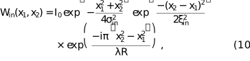
$[\eqalignno{ W_{\rm{in}}({x_1},{x_2}) = {}& {I_0}\exp \left({ - {{x_1^2 + x_2^2} \over {4\sigma _{\rm{in}}^2}}} \right) \exp \left({{{ - {{\left({{x_2} - {x_1}} \right)}^2}} \over {2\xi _{\rm{in}}^2}}} \right) \cr& \times \exp \left({{{ - i\pi \left({x_2^2 - x_1^2} \right)} \over {\lambda R}}} \right), & (10) }]$

where σ_in is the r.m.s. beam width of the incident beam, ξ_in is its spatial coherence length, and R is the radius of curvature of a Gaussian beam. Throughout this paper, the coherence length is defined as the r.m.s. width of the CCF, which is extracted by Gaussian fitting of the simulated curve. For profiles that deviate significantly from a Gaussian shape, the coherence length is alternatively evaluated using its width at 0.6 of the peak intensity. As a theoretical benchmark, ξ_in is calculated using the simulation method detailed in Section 2.2. Substituting equation (10) into the definition of the ICSD,

$[G\left({\Delta x}\right) = {I_0}\sqrt{2\pi} \,{\sigma _{\rm{in}}}\exp \left({{{ - \Delta {x^2}} \over {2\xi _{\rm{in}}^2}}} \right)\exp \left({{{ - \Delta {x^2}} \over {8\sigma _{\rm{in}}^2}}} \right). \eqno(11) ]$

Equation (11) demonstrates that for a GSM beam the visibility curve measured by XGI remains Gaussian. Let ξ_meas be the r.m.s. width of this measured visibility curve. We have the relationship linking the measured visibility width, the beam coherence length, and the beam size,

$[{1 \over {\xi _{\rm meas}^2}} = {1 \over {\xi _{\rm{in}}^2}} + {1 \over {4\sigma _{\rm{in}}^2}}. \eqno(12)]$

This equation indicates that the XGI-measured visibility width is always smaller than the coherence length (ξ_meas < ξ_in). This difference becomes significant when σ_in is comparable with or smaller than ξ_in. In our previous work (Lu et al., 2025), we attributed this difference primarily to the breakdown of spatial shift invariance. In this paper, we reveal that the finite beam size also affects the measurement.

A fully coherent Gaussian beam is a limiting case of the GSM. Its CCF is a constant of 1, |μ_in| = 1. Equation (11) then reduces to

$[G\left({\Delta x} \right) = {I_0}\sqrt{2\pi}\, {\sigma _{\rm{in}}}\exp \left({{{ - \Delta {x^2}} \over {8\sigma _{\rm{in}}^2}}} \right). \eqno(13)]$

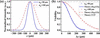
According to equation (13), the XGI-measured r.m.s. width of the visibility curve ξ_meas = 2σ_in. It is affected by the finite size of the beam-intensity profile. Fig. 3 illustrates the numerical simulation results for this extreme case, which is only for theoretical validation purposes rather than a physical experiment. The XGI-measured visibility still exhibits a pronounced drop even for a fully coherent incident beam, rather than a horizontal line of constant 1. However, the visibility curve extracted from the simulated interferograms matches the analytical prediction [equation (13)] very well. We simulate two cases in Fig. 3. The fitted visibility widths agree with the theoretical value (2σ_in) as expected.

Figure 3
(a) Incident intensity profiles of two fully coherent Gaussian beams. The r.m.s. widths are σ_in = 50 µm (blue solid line) and σ_in = 100 µm (red dashed line). (b) Visibility curves extracted from simulated XGI interferograms (blue circles and red triangles) and analytical prediction based on equation (13)

(blue solid and red dashed lines).

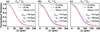
We also run numerical simulations for general GSM beams to validate our theory (Fig. 4). The visibility curves extracted from the simulated XGI interferograms (blue open circles) agree well with the theoretical curve calculated via the ICSD formulation (red solid lines) for all cases. Crucially, as the beam coherence increases from Fig. 4(a) to Fig. 4(c), the XGI-measured visibility deviates more from the theoretical CCF (gray dashed lines). This distinction becomes particularly important for DLSRs, in which X-ray beams possess high spatial coherence, ξ_in ≥ σ_in. In these cases, the XGI-measured visibility curve clearly becomes significantly narrower than the theoretical CCF.

Figure 4
Validation of the ICSD under different conditions at the grating plane: (a) σ_in > ξ_in, (b) σ_in = ξ_in, and (c) σ_in < ξ_in. The blue open circles represent XGI-measured visibility curves from simulations. The red solid lines denote analytical predictions based on the ICSD. The gray dashed lines show the theoretical CCF for reference. The extracted visibility width ξ_meas, the theoretical input coherence length ξ_in, and the corrected coherence length ξ_corr calculated via equation (12)

are annotated.

2.3.2. The real SR source

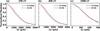
We simulate these real sources using the CMD method described in Section 2.2. The source parameters are from the Hefei Advanced Light Facility (HALF) (Sun & Feng, 2024 ; Lu et al., 2025) at typical photon energies of 250 eV, 400 eV, and 1000 eV. As shown in Fig. 5, the simulated visibility curves agree with the theoretical ICSD curves for all three cases.

Figure 5
Validation of the ICSD using real SR sources. Panels (a), (b), and (c) show visibility curves of HALF corresponding to photon energies of 250 eV, 400 eV, and 1000 eV, respectively. The blue open circles represent the visibility extracted from the full wave optical simulations of the XGI. The red solid lines denote the normalized ICSD for each photon energy.

It should be noted that equation (12) is derived under the GSM approximation. We compared the visibility widths measured by XGI (ξ_meas) with the corrected coherence lengths (ξ_corr) by equation (12) in Table 1. As the photon energy decreases from 1000 eV to 250 eV, the source approaches the diffraction limit. The initial relative difference (Δξ/ξ) between the XGI-measured visibility width and the theoretical coherence length ranges from 17.2% to 33.7%. By applying equation (12), the difference is reduced to below 10% for both the 400 eV and 1000 eV cases.

Table 1
Coherence lengths from XGI before and after the correction

Source condition	ξ_in (µm)	ξ_meas (µm)	Initial difference	ξ_corr (µm)	Remaining difference
250 eV	1837.1	1218.9	33.7%	1528.8	16.8%
400 eV	1173.3	884.3	24.6%	1059.0	9.7%
1000 eV	512.4	424.4	17.2%	463.6	9.5%
400 eV, 0.1×-size	2080.8	1033.9	50.3%	1349.9	35.1%

However, for 250 eV, the difference remains 16.8%. For further investigation, we introduced an extreme case by decreasing the electron beam to 0.1× its initial size at 400 eV. The beam divergence and lattice parameters were kept constant, and the emittance was scaled proportionally. As shown in the last line of Table 1, it yields a remaining difference of 35.1% after correction. The underlying reason becomes clear when recalling that equation (12) relies on the Schell-model assumption. As demonstrated in our previous work (Lu et al., 2025), deeply diffraction-limited sources can significantly violate the Schell-model condition at the grating plane. Consequently, this correction becomes insufficient for these extreme conditions.

3. XGI for source size measurement

Recent commissioning results from DLSRs, such as the Advanced Photon Source-Upgrade (APS-U) (Shi et al., 2025) and the High Energy Photon Source (HEPS) (Li, 2025; Jiao et al., 2018 ), have highlighted an interesting phenomenon. Although the visibility width measured by XGI is significantly smaller than the coherence length, XGI can still measure the source size with tolerable error. We will use our theory to explain this observation. As in the previous section, we start with the well studied GSM source. The GSM source can help us find a clue to a satisfactory explanation when discussing the real SR source.

3.1. The GSM source

In the source plane, the CSD of the GSM can be written as

$[W_{\rm{s}}(\alpha_1,\alpha_2) = \sqrt{I_{\rm{s}}\left(\alpha_1\right) \, I_{\rm{s}}\left(\alpha_2\right)} \, \mu\left(\alpha_2-\alpha_1\right), \eqno(14)]$

where the source intensity is I_s(α) = I_s0exp[−α²/(2σ_s²)], and the CCF is μ_s(α₂ − α₁) = exp[−(α₂ − α₁)²/(2ξ_s²)]. Here, σ_s denotes the r.m.s. source size and ξ_s is the source coherence length. It is convenient to express the CSD in terms of the mean coordinate $[\bar\alpha]$ = (α₂ + α₁)/2 and difference coordinate Δα = α₂ − α₁,

$[{W_{\rm{s}}}(\bar\alpha, \Delta \alpha) = {I_{\rm{s}}}\left({\bar\alpha } \right) \, \mu_{\rm{s}}^{\prime}\left({\Delta \alpha } \right), \eqno(15)]$

where we define an effective CCF $[\mu_{\rm{s}}^{\prime}(\Delta\alpha)]$ = exp{−Δα² / 2[1/(4σ_s²) + 1/(ξ_s²)]}. Equation (15) reflects a Schell-model separability condition in mean and difference coordinates.

After propagating a distance D, the CSD at the grating plane relates to the CSD from the source via the far-field approximation, which assumes that the propagation distance is approximately equal to the wavefront radius of curvature (D ≃ R) (Goodman, 2015),

$[\eqalignno{ {W_{\rm{in}}}\left({\bar x, \Delta x} \right) \simeq {}& {{{\exp\left( - i\psi\right)}} \over {\lambda D}}\int\!\!\!\int {W_{\rm{s}}}(\bar \alpha, \Delta \alpha) \cr& \times \exp \left [{{{i2\pi } \over {\lambda D}}\left({\bar x \Delta \alpha + \bar \alpha \Delta x} \right)} \right] \,{\rm{d}}\bar\alpha\,{\rm{d}}\Delta\alpha , & (16) }]$

where ψ = π(x₂² − x₁²)/(λD) is a phase factor. By substituting equation (15) into equation (16) and separating the integrals over $[\bar\alpha]$ and Δα, the propagated CSD factorizes as

$[{W_{\rm{in}}}\left({\bar x, \Delta x} \right) = {\exp\left( - i\psi\right)} \, F\left\{ {{I_{\rm{s}}}\left({\bar \alpha } \right)} \right\}\Big| _{f\,=\,{{\Delta x}/{\lambda D}}} \ M\left({\bar x } \right), \eqno(17)]$

where $[M(\bar{x})]$ = $[1/(\lambda D)\textstyle\int\mu_{\rm{s}}^{\prime}(\Delta\alpha)\exp[i2\pi\bar{x}\Delta\alpha/(\lambda D)]\,{\rm{d}}\Delta\alpha]$ . Substituting equation (17) into the definition of the ICSD, we obtain

$[G\left({\Delta x} \right) = K \left| {F\left\{ {{I_{\rm{s}}}\left({\bar\alpha } \right)} \right\}\Big| _{f\,=\,{{\Delta x}/{\lambda D}}}} \right|, \eqno(18)]$

where K = $[|\textstyle \int M(\bar x)\,{\rm{d}}\bar x\,|]$ is independent of Δx, F denotes the Fourier transform, and f is the spatial frequency.

Equation (18) shows that the normalized visibility curve measured by XGI is equivalent to the normalized Fourier transform of the source intensity profile. The Fourier transform of a Gaussian source intensity I_s(α) is also Gaussian. Denoting the r.m.s. width of the XGI-measured visibility curve as ξ_meas, equation (18) leads to

$[\sigma_{\rm{s}} = {{\lambda D} \over {2\pi{\xi_{\rm meas}}}}. \eqno(19)]$

Equation (19) is identical in form to the formula used in the recent study (Shi et al., 2025). It implies that the Schell-model separability condition in mean and difference coordinates determines the validity of XGI for measurement of a conventional coherence length.

3.2. The real SR source

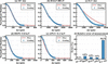
We performed numerical simulations using the design parameters of APS-U at 11.3 keV, HEPS at 13.8 keV, and HALF at 400 eV. The key simulation parameters of HEPS and APS-U are summarized in Table 2 (Shi et al., 2025; Jiao et al., 2018; Borland & Blednykh, 2018 ), while those for HALF are the same as in our previous work (Lu et al., 2025). In addition, we introduced two limiting conditions. We multiplied the designed HALF electron beam size by factors of 10 and 0.1, respectively, following the same scaling principle as in Section 2.3.2. The photon energy remains at 400 eV. The 10×-size case represents a nearly incoherent source. The 0.1×-size case has been simulated in Section 2.3.2. We first use equation (18) to compare the XGI-measured visibility curve with the Fourier transform of the source intensity for each case [Figs. 6(a)–6(e)]. Then we apply equation (19) to calculate the source size and evaluate the relative error (Δσ_s/σ_s), as summarized in Fig. 6(f).

Table 2
Key parameters of the storage rings and undulators for the numerical simulations

Parameter	HEPS	APS-U
Electron beam energy (GeV)	6.0	6.0
Current (A)	0.20	0.05
Horizontal emittance (m rad)	2.728 × 10⁻¹¹	4.368 × 10⁻¹¹
Vertical emittance (m rad)	2.76 × 10⁻¹²	3.36 × 10⁻¹²
Energy spread	1.1 × 10⁻³	1.56 × 10⁻³
Undulator period (m)	0.0199	0.027
Undulator length (m)	4	2.349
Propagation distance D (m)	44.326	36.5
Grating period (µm)	1.2	3.4

Figure 6
Comparison between the simulated XGI visibility curves (blue open circles) and the modulus of the theoretical Fourier transform of the actual source intensity (red solid lines) for (a) 10×-size source, (b) HALF at 400 eV, (c) 0.1×-size source, (d) HEPS at 13.8 keV, and (e) APS-U at 11.3 keV. (f) The relative error of the source size measurement (Δσ/σ) using equation (19)

for each corresponding case.

The simulated visibility curves in Figs. 6(a), 6(b), 6(d), and 6(e) match the Fourier transforms of the source intensities. However, for the 0.1×-size case [Fig. 6(c)], a significant discrepancy exists between the two curves. This direct deviation indicates that the theoretical approximation in equation (18) fails due to CSD non-separability.

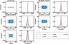
To visually evaluate this non-separability property, we examine the full CSD profiles. If the source satisfies the Schell-model separability property in mean and difference coordinates, its CSD is separable, as shown in equation (15). To evaluate the separability for |W_s( $[\bar\alpha]$ , Δα)|, we examine the normalized CSD profiles extracted at any arbitrary position $[\bar\alpha]$ . If |W_s( $[\bar\alpha]$ , Δα)| is a separable function of $[\bar\alpha]$ and Δα, these profiles should be independent of $[\bar\alpha]$ and overlay perfectly. Fig. 7 shows the results for the same five cases in Fig. 6. In each case, the left panel shows the vertical CSD modulus |W_s( $[\bar\alpha]$ , Δα)|. The right panel displays the corresponding normalized CSD profiles extracted at various positions $[\bar\alpha]$ in the range [−1.5σ, 1.5σ], where σ is the r.m.s. width of |W_s( $[\bar\alpha]$ , 0)|.

Figure 7
(a)–(e) Vertical CSD modulus |W_s( $[\bar\alpha]$ , Δα)| in the source plane (left) and the corresponding normalized profiles extracted at various positions $[\bar\alpha]$ in the range [−1.5σ, 1.5σ] (right). Here, σ denotes the r.m.s. size of the profile at Δα = 0. Cases: (a) 10×-size source, (b) HALF at 400 eV, (c) 0.1×-size source, (d) HEPS at 13.8 keV, and (e) APS-U at 11.3 keV.

As shown in Fig. 7(a), the normalized CSD profiles have the same shape at all evaluated $[\bar\alpha]$ positions for the 10×-size source, indicating the separability of the CSD and leading to a negligible relative error of 0.1% [Fig. 6(f)]. For real SR sources [Figs. 7(b), 7(d), and 7(e)], the extracted profiles still largely overlay in the central region, indicating that the separability condition is approximately maintained for the three sources. As a result, equation (19) remains effective, yielding acceptable relative errors of 4.0% for HALF, 6.0% for HEPS, and 3.0% for APS-U.

However, for the 0.1×-size limiting case [Fig. 7(c)], as the evaluation position moves away from the center, the normalized profiles transit from a single peak at the center to a split bimodal structure at the outer edges. This variation and the large error of 38.2% show that the Schell-model separability approximation fails. The simple formula in equation (19) becomes inadequate for such a deeply diffraction-limited source. It is worth noting that this extreme case is close to the radiation from a single electron, a theoretical bound that real storage rings will rarely reach in practice.

4. Conclusion

In this paper, we have explained the physical mechanism of XGI using the framework of wave optics. We have shown that, under the assumption of a global quadratic phase for the incident beam, the XGI-measured visibility is the normalized ICSD. The ICSD is a global metric for spatial coherence. It differs from the local CCF. This distinction determines the discrepancy between the XGI-measured visibility width and the coherence length conventionally defined in DLSR measurements. As an example, we showed a simple correction for the ideal GSM beams. Furthermore, by clarifying the exact physical quantity the XGI measures, we explained why the XGI yields a reliable characterization of source size.

Overall, the theoretical insights provide a foundation for the applications of the XGI method. The proposed correction and the analysis of source size characterization offer practical tools for evaluating the electron beam emittance. They will help to optimize and utilize next-generation SR facilities. The theoretical results proposed in this paper are not limited to the XGI. There are many other experimental methods that can be used to measure the conventional coherence length and the source size. Many of them rely on interferometry. Usually, they assume the Schell-model separability of the CSD from the source. The theoretical results in this paper show that, for DLSR, these methods should be revisited, especially when the electron beam size or divergence is much smaller than the intrinsic emission of a single electron. Besides, the longer the wavelength emitted from the electron beam, the more care is needed. Therefore, the question raised and the results obtained in this paper are also helpful for other interferometric methods.

Acknowledgements

We thank the USTC Supercomputing Center for computing resource. We also acknowledge Dr Ming Li (from HEPS) for the invaluable discussions.

Conflict of interest

The authors declare no conflicts of interest.

Data availability

Data underlying the results presented in this paper are not publicly available at this time but may be obtained from the authors upon reasonable request.

Funding information

The following funding is acknowledged: Fundamental Research Funds for the Central Universities (WK2310000120); University of Science and Technology of China (USTC) under Grant No. USTC-NSRL202507 (KY3040000900).

References

Alaimo, M. D., Anania, M. P., Artioli, M., Bacci, A., Bellaveglia, M., Ciocci, F., Chiadroni, E., Cianchi, A., Dattoli, G., Di Pirro, G., Ferrario, M., Gatti, G., Giannessi, L., Manfredda, M., Martucci, R., Mostacci, A., Paroli, B., Petralia, A., Petrillo, V., Pompili, R., Potenza, M. A., Quattormini, M., Rau, J., Redoglio, D., Rossi, A. R., Serafini, L., Surrenti, V., Torre, A., Vaccarezza, C. & Villa, F. (2014). Opt. Express 22, 30013–30023. CrossRef PubMed Google Scholar
Bagschik, K., Frömter, R., Müller, L., Roseker, W., Bach, J., Staeck, P., Thönnißen, C., Schleitzer, S., Berntsen, M. H., Weier, C., Adam, R., Viefhaus, J., Schneider, C. M., Grübel, G. & Oepen, H. P. (2016). Opt. Express 24, 23162–23176. CrossRef CAS PubMed Google Scholar
Bagschik, K., Schneider, M., Wagner, J., Buss, R., Riepp, M., Philippi-Kobs, A., Müller, L., Roseker, W., Trinter, F., Hoesch, M., Viefhaus, J., Eisebitt, S., Grübel, G., Oepen, H. P. & Frömter, R. (2020). Opt. Lett. 45, 5591–5594. CrossRef PubMed Google Scholar
Bei, M., Borland, M., Cai, Y., Elleaume, P., Gerig, R., Harkay, K., Emery, L., Hutton, A., Hettel, R., Nagaoka, R., Robin, D. & Steier, C. (2010). Nucl. Instrum. Methods Phys. Res. A 622, 518–535. CrossRef Google Scholar
Borland, M. & Blednykh, A. (2018). Report BNL-209801-2018-PUCP. Brookhaven National Laboratory, Upton, NY, USA. Google Scholar
Chubar, O. & Celestre, R. (2019). Opt. Express 27, 28750–28759. CrossRef PubMed Google Scholar
Chubar, O. & Elleaume, P. (1998). Proceedings of the Sixth European Particle Accelerator Conference (EPAC'98), 22–26 June 1998, Stockholm, Sweden, pp. 1177–1179. THP01G. Google Scholar
Chushkin, Y. & Zontone, F. (2025). IUCrJ 12, 280–287. Web of Science CrossRef CAS PubMed IUCr Journals Google Scholar
Cloetens, P., Guigay, J. P., De Martino, C., Baruchel, J. & Schlenker, M. (1997). Opt. Lett. 22, 1059–1061. CrossRef PubMed CAS Web of Science Google Scholar
Coïsson, R. & Marchesini, S. (1997). J. Synchrotron Rad. 4, 263–266. CrossRef Web of Science IUCr Journals Google Scholar
Duarte, J., Gonzalez, A. I., Cassin, R., Nicolas, R., Kholodstova, M., Boutu, W., Fajardo, M. & Merdji, H. (2021). Opt. Lett. 46, 1764–1767. CrossRef PubMed Google Scholar
Friberg, A. T. & Sudol, R. J. (1982). Opt. Commun. 41, 383–387. CrossRef Web of Science Google Scholar
Geloni, G., Kocharyan, V. & Saldin, E. (2015). J. Synchrotron Rad. 22, 288–316. Web of Science CrossRef CAS IUCr Journals Google Scholar
Glass, M. (2017). PhD thesis, Université Grenoble Alpes, France. Google Scholar
Glass, M. & Sanchez del Rio, M. (2017). Europhys. Lett. 119, 34004. Web of Science CrossRef Google Scholar
Goodman, J. W. (2015). Statistical optics. Hoboken: John Wiley & Sons. Google Scholar
Goodman, J. W. (2017). Introduction to Fourier Optics 4th ed. W. H. Freeman and Company. Google Scholar
Gori, F., Santarsiero, M., Simon, R., Piquero, G., Borghi, R. & Guattari, G. (2003). J. Opt. Soc. Am. A 20, 78–84. CrossRef Google Scholar
Guigay, J.-P., Zabler, S., Cloetens, P., David, C., Mokso, R. & Schlenker, M. (2004). J. Synchrotron Rad. 11, 476–482. Web of Science CrossRef CAS IUCr Journals Google Scholar
Jiao, Y., Xu, G., Cui, X.-H., Duan, Z., Guo, Y.-Y., He, P., Ji, D.-H., Li, J.-Y., Li, X.-Y., Meng, C., Peng, Y.-M., Tian, S.-K., Wang, J.-Q., Wang, N., Wei, Y.-Y., Xu, H.-S., Yan, F., Yu, C.-H., Zhao, Y.-L. & Qin, Q. (2018). J. Synchrotron Rad. 25, 1611–1618. Web of Science CrossRef IUCr Journals Google Scholar
Khubbutdinov, R., Geloni, G., Saldin, E. & Bagschik, K. (2024). Opt. Express 32, 47810. CrossRef PubMed Google Scholar
Khubbutdinov, R., Menushenkov, A. P. & Vartanyants, I. A. (2019). J. Synchrotron Rad. 26, 1851–1862. Web of Science CrossRef CAS IUCr Journals Google Scholar
Kim, K.-J. (1986). Proc. SPIE 0582, 2–9. CrossRef CAS Google Scholar
Klementiev, K. & Chernikov, R. (2014). Proc. SPIE 9209, 60–75. Google Scholar
Leitenberger, W., Kuznetsov, S. & Snigirev, A. (2001). Opt. Commun. 191, 91–96. CrossRef CAS Google Scholar
Li, M. (2025). Private communication. Google Scholar
Lin, J. J., Paterson, D., Peele, A. G., McMahon, P. J., Chantler, C. T., Nugent, K. A., Lai, B., Moldovan, N., Cai, Z., Mancini, D. C. & McNulty, I. (2003). Phys. Rev. Lett. 90, 074801. CrossRef PubMed Google Scholar
Lu, Y., Gao, K., Zhao, S., Wang, Q. & Hu, L. (2025). Opt. Lett. 50, 6746–6749. CrossRef PubMed Google Scholar
Marathe, S., Shi, X., Wojcik, M. J., Kujala, N. G., Divan, R., Mancini, D. C., Macrander, A. T. & Assoufid, L. (2014). Opt. Express 22, 14041–14053. CrossRef PubMed Google Scholar
Munro, P. R., Ignatyev, K., Speller, R. D. & Olivo, A. (2010). Opt. Express 18, 19681–19692. CrossRef PubMed Google Scholar
Narayanan, T., Chèvremont, W. & Zinn, T. (2025). J. Appl. Cryst. 58, 535–542. Web of Science CrossRef CAS IUCr Journals Google Scholar
Nugent, K. A. & Trebes, J. E. (1992). Rev. Sci. Instrum. 63, 2146–2151. CrossRef CAS Google Scholar
Pfeiffer, F. (2017). Nat. Photon. 12, 9–17. Web of Science CrossRef Google Scholar
Pfeiffer, F., Bunk, O., Schulze-Briese, C., Diaz, A., Weitkamp, T., David, C., van der Veen, J. F., Vartanyants, I. & Robinson, I. K. (2005). Phys. Rev. Lett. 94, 164801. Web of Science CrossRef PubMed Google Scholar
Qi, J. C., Ye, L. L., Chen, R. C., Xie, H. L., Ren, Y. Q., Du, G. H., Deng, B. & Xiao, T. Q. (2014). Acta Phys. Sin. 63, 104202. Google Scholar
Samadi, N., Shi, X., Dallin, L. & Chapman, D. (2020). Phys. Rev. Accel. Beams 23, 024801. CrossRef Google Scholar
Sanchez del Rio, M., Canestrari, N., Jiang, F. & Cerrina, F. (2011). J. Synchrotron Rad. 18, 708–716. Web of Science CrossRef CAS IUCr Journals Google Scholar
Sanchez del Rio, M., Celestre, R., Reyes-Herrera, J., Brumund, P. & Cammarata, M. (2022). J. Synchrotron Rad. 29, 1354–1367. Web of Science CrossRef CAS IUCr Journals Google Scholar
Shi, X., Lin, Y.-C., Zhao, J., Toellner, T., Hu, M. Y., Seifert, S., Lee, B., Grizolli, W., Wojcik, M. J., Rebuffi, L., Assoufid, L. & Sajaev, V. (2025). J. Synchrotron Rad. 32, 1152–1161. Web of Science CrossRef CAS IUCr Journals Google Scholar
Siano, M., Geloni, G., Paroli, B., Butti, D., Lefèvre, T., Mazzoni, S., Trad, G., Iriso, U., Nosych, A. A., Torino, L. & Potenza, M. A. C. (2023). J. Synchrotron Rad. 30, 217–226. CrossRef CAS IUCr Journals Google Scholar
Siano, M., Paroli, B., Potenza, M. A. C., Teruzzi, L., Iriso, U., Nosych, A. A., Solano, E., Torino, L., Butti, D., Goetz, A., Lefevre, T., Mazzoni, S. & Trad, G. (2022). Phys. Rev. Accel. Beams 25, 052801. CrossRef Google Scholar
Skopintsev, P., Singer, A., Bach, J., Müller, L., Beyersdorff, B., Schleitzer, S., Gorobtsov, O., Shabalin, A., Kurta, R. P., Dzhigaev, D., Yefanov, O. M., Glaser, L., Sakdinawat, A., Grübel, G., Frömter, R., Oepen, H. P., Viefhaus, J. & Vartanyants, I. A. (2014). J. Synchrotron Rad. 21, 722–728. Web of Science CrossRef CAS IUCr Journals Google Scholar
Sun, Z. & Feng, D. (2024). Chin. Phys. Lett. 41, 037303. Google Scholar
Takayama, Y., Tai, R. Z., Hatano, T., Miyahara, T., Okamoto, W. & Kagoshima, Y. (1998). J. Synchrotron Rad. 5, 456–458. Web of Science CrossRef CAS IUCr Journals Google Scholar
Takeda, M., Ina, H. & Kobayashi, S. (1982). J. Opt. Soc. Am. 72, 156–160. CrossRef Web of Science Google Scholar
Tanaka, T. & Kitamura, H. (2001). J. Synchrotron Rad. 8, 1221–1228. Web of Science CrossRef CAS IUCr Journals Google Scholar
Tang, R., Organista, C., Goethals, W., Stolp, W., Stampanoni, M., Aelterman, J. & Boone, M. N. (2023). Opt. Express 31, 1677–1691. CrossRef CAS PubMed Google Scholar
Trebushinin, A., Geloni, G., Serkez, S., Khubbutdinov, R. & Saldin, E. (2024). Phys. Rev. Accel. Beams 27, 032802. CrossRef Google Scholar
Vartanyants, I. A. (2024). Phys. Rev. A 110, 063531. CrossRef Google Scholar
Vartanyants, I. A. & Singer, A. (2020). Synchrotron Light Sources and Free-Electron Lasers: Accelerator Physics, Instrumentation and Science Applications pp. 987–1029. Cham: Springer International Publishing. Google Scholar
Yashiro, W., Noda, D. & Kajiwara, K. (2018). Opt. Express 26, 1012–1027. CrossRef CAS PubMed Google Scholar
Zhang, W., Zhu, D., Sui, Y., Yue, J., Cao, J. & He, J. (2023). J. Synchrotron Rad. 30, 910–916. CrossRef CAS IUCr Journals Google Scholar

This is an open-access article distributed under the terms of the Creative Commons Attribution (CC-BY) Licence, which permits unrestricted use, distribution, and reproduction in any medium, provided the original authors and source are cited.

JOURNAL OF
SYNCHROTRON
RADIATION

ISSN: 1600-5775

Volume 34| Part 1| January 2027|

https://doi.org/10.1107/S1600577526010544

Open

access

Format		BIBTeX
		EndNote
		RefMan
		Refer
		Medline
		CIF
		SGML
		Plain Text
		Text

Format		BIBTeX
		EndNote
		RefMan
		Refer
		Medline
		CIF
		SGML
		Plain Text
		Text

research papers\(\def\hfill{\hskip 5em}\def\hfil{\hskip 3em}\def\eqno#1{\hfil {#1}}\)

Theoretical explanation of spatial coherence and source size characterization by X-ray grating interferometry

1. Introduction

2. General theory of XGI

2.1. XGI under general conditions

2.2. Numerical simulation scheme

2.3. Application of the theory to special cases

2.3.1. The GSM beam

2.3.2. The real SR source

3. XGI for source size measurement

3.1. The GSM source

3.2. The real SR source

4. Conclusion

Acknowledgements

Conflict of interest

Data availability

Funding information

References

research papers