Iterative phase retrieval in macromolecular crystal diffraction using the gradients of intensities

Bielfeldt, S.; Yefanov, O.; Mnich, M.; Chapman, H.N.

doi:10.1107/S1600576726008137

research papers

JOURNAL OF
APPLIED
CRYSTALLOGRAPHY

ISSN: 1600-5767

Volume 59| Part 6| December 2026|

https://doi.org/10.1107/S1600576726008137

Open

access

Iterative phase retrieval in macromolecular crystal diffraction using the gradients of intensities

Sebastian Bielfeldt,^a,^b ^* Oleksandr Yefanov,^a Matthias Mnich ^b and Henry N. Chapman ^a,^c,^d

^aCenter for Free-Electron Laser Science CFEL, Deutsches Elektronen-Synchrotron DESY, Notkestr. 85, 22607 Hamburg, Germany, ^bHamburg University of Technology, Institute for Algorithms and Complexity, Hamburg, Germany, ^cThe Hamburg Centre for Ultrafast Imaging, Luruper Chaussee 149, 22761 Hamburg, Germany, and ^dDepartment of Physics, University of Hamburg, Luruper Chaussee 149, 22761 Hamburg, Germany
^*Correspondence e-mail: [email protected]

Edited by S. Boutet, SLAC National Accelerator Laboratory, Menlo Park, USA (Received 15 April 2026; accepted 6 August 2026; online 17 October 2026)

Iterative phase retrieval (IPR) offers a model-independent route to crystallographic structure determination but is fundamentally limited by the sampling of the diffraction pattern at Bragg positions. Consequently, conventional IPR methods typically rely on a high solvent fraction (>70%) to sufficiently constrain the solution, a condition met by only a small fraction of protein crystals. This work investigates a magnitude-and-gradient IPR algorithm that overcomes this undersampling barrier by exploiting the local intensity gradients ∇I(q) observable in the diffraction patterns of finite crystals. By incorporating the gradients of the molecular transform alongside Bragg intensities, the phase problem is converted from an underdetermined system of equations to one that is overdetermined by a factor of two. Tests on simulated diffraction data for proteins in space group P1 demonstrate that the algorithm successfully reconstructs electron densities across a wide range of solvent fractions, including densely packed crystals where standard algorithms fail. Furthermore, the approach proves robust under experimentally relevant conditions, tolerating significant Poissonian noise and the loss of low-resolution terms due to a beamstop when coupled with approximate real-space support constraints. These results indicate that leveraging the fine structure of Bragg peaks at coherent X-ray sources can significantly extend the applicability of ab initio phasing.

Keywords: iterative phase retrieval; ab initio phasing; macromolecular crystallography; nanocrystals.

1. Introduction

Diffraction from 3D crystals produces distinct intensity maxima known as Bragg peaks. In X-ray crystallography, the integrated counts in these peaks are used to perform a Fourier synthesis of the crystal electron density. At the heart of this process lies the long-standing phase problem: recovering the phases $[\varphi({\bf q})]$ of the structure factors $[F({\bf q})]$ from the measured intensities $[I({\bf q})]$ at reciprocal-space positions $[{\bf q}]$ . While a wide range of computational and experimental methods have been developed to address this challenge, the fundamental limitation remains that only intensities are directly measured. Without phase information, the inverse Fourier transform $[{\cal F}^{-1}]$ of the measured intensities yields the autocorrelation function of the molecular electron density $[\rho_{\rm {mol}}({\bf r})]$ ,

$[{\cal F}^{-1}[|F_{\rm mol}({\bf q})|^2] = A_{\rm mol}(\Delta {\bf r}),\eqno(1)]$

with the interpoint distance $[\Delta{\bf r}]$ and the autocorrelation function

$[A_{\rm {mol}}(\Delta{\bf r}) = \rho_{\rm {mol}}({\bf r})\star\rho_{ {\rm mol}}(-{\bf r}) = \int\rho_{\rm {mol}}({\bf r})\rho_{\rm {mol}}(\Delta {\bf r}+{\bf r})\,{\rm d}{\bf r}.\eqno(2)]$

Here, $[\star]$ denotes the convolution operation and $[{\bf r}]$ is the real-space coordinate. The autocorrelation function of a compact object is centrosymmetric even when the object is not; at the same time it has twice the extent of the object itself. For example, the convolution of the unit cube with itself is non-zero in a cube of side length 2, containing all pair correlation vectors that can exist in the unit cube. The autocorrelation function of an infinite crystal is also of infinite extent. However, the infinite crystal and its autocorrelation function share the same periodicity, so the autocorrelation generally extends into neighboring unit cells and only the central part not overlapped by neighboring cells is unique. Because protein crystals lack inversion symmetry, the autocorrelation acquires an additional center of inversion relative to the crystal, so that within one unit cell the unique information is confined to a fraction of the cell. This is known as the Patterson function (Patterson, 1934 ), which can be thought of as an aliased version of the autocorrelation function. In this case, one cannot distinguish intramolecular pair correlations from intermolecular ones, leading to ambiguity.

This ambiguity would vanish if the molecular transform were sampled twice as finely as the Bragg spacing, as this would fully determine the autocorrelation function of the molecule (Shannon, 1949 ; Sayre, 1952 ). In two and three dimensions, the measurement of the complete autocorrelation function of the compact object is usually sufficient to uniquely determine all phases (Miao et al., 1998 ), as can be quantified by the constraint ratio of the number of independent intensity measurements to the number of coefficients required to describe the electron density of the molecule, $[\rho_{\rm {mol}}({\bf r})]$ (Elser & Millane, 2008 ). In a molecular crystal with only translational symmetry, any increase in the unit cell in comparison with the size of the molecular unit means an increase in solvent fraction. This increases the number of Bragg peaks relative to the molecular transform compared with a more tightly packed crystal. That is, the molecular transform is more finely sampled in reciprocal space. We illustrate this in Fig. 1, where we compare the diffraction patterns of a single duck molecule with those of duck crystals with high and low solvent fractions. The transform of the single duck is sampled more finely when the solvent occupies a larger fraction of the unit-cell volume, approaching the limit of twice as many Fourier constraints per dimension when the unit-cell width is at least double the molecular extent in that direction.

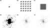Figure 1
The top row (a, b, c) shows the duck-shaped `density' in black as well as the outline of the autocorrelation function in gray. The bottom row (d, e, f) shows the center of the Fourier transform of the respective `densities' above, where the intensity in the leftmost plot is enhanced by a factor of 1000 compared with the maximum of the other two plots. From left to right, we show a single duck (a), a $[5\times 5]$ duck crystal with wide solvent spacing (b) and a $[5\times 5]$ duck crystal with tight solvent spacing (c). In the case of (b), the autocorrelation function fits well within the unit cell, whereas there is significant overlap in (c). As the unit cell contains more empty/solvent space, the duck's Fourier transform is thus sampled more finely in (e) than in (f). One can also see how the lattice peaks of (e) and (f) match the high- and low-intensity regions of the single-duck intensities in (c).

A potential approach to reconstruct $[\rho_{\rm {mol}}({\bf r})]$ is to use iterative projection algorithms (Millane, 1990 ; Marchesini, 2007 ; Millane & Lo, 2013 ; Barnett et al., 2024 ). Here, prior information about the object is used to construct constraint sets which $[\rho_{\rm {mol}}({\bf r})]$ must satisfy. This includes the measured $[I({\bf q}_{hk\ell})]$ , but may also incorporate real-space information, such as the value distribution of the electron density, the object's approximate shape or the atomicity of the density (for high-resolution diffraction). Such algorithms explore the space of possible electron densities to find the intersection of constraint manifolds. Typically, this involves alternating between reciprocal space – where the object's transform must match the measured structure-factor magnitudes – and real space, where the density is constrained by the assumed molecular support, density histograms, atomicity or positivity of the density. The conceptual foundation of iterative phase retrieval (IPR) lies in the Gerchberg–Saxton (Gerchberg & Saxton, 1972 ) and error reduction algorithms (Fienup, 1982 ; Griffin & Lim, 1984 ), which alternate between enforcing known Fourier magnitudes and real-space constraints. While these algorithms guarantee a reduction (or non-increase) of the error, they are prone to stagnation in local minima and show poor convergence in the presence of noise. Algorithms such as the hybrid input–output method (Fienup, 1982) forgo guarantees of converging to the true solution, in exchange for the ability to escape local minima. Later projection-based schemes – including the difference map (Elser, 2003 ), relaxed averaged alternating reflections (Luke, 2005 ), relaxed–reflect–reflect (Elser, 2025 ) and alternating direction method of multipliers (ADMM) (Wen et al., 2012 ) – provided tunable parameters, more general projection formulations and stable convergence behavior.

These algorithms are designed for only two constraint sets. A way to combine more than two such sets into these algorithms was introduced with the `divide and concur' method (Gravel & Elser, 2008 ). This approach uses multiple copies of the electron density concatenated into a single state vector. One projection operation for the algorithm, the divide projection, is formed by projecting each copy, or replica, within the state vector onto its corresponding individual constraint set. The second operation, the concur projection, is to enforce consistency between all replicas, such as by replacing each replica with their average. Through this approach, an arbitrary number of constraint sets can be seamlessly integrated into the aforementioned algorithms. Elser (2013 ) applied this approach to demonstrate the possibility of using the intensity gradients measured at reciprocal-lattice points as additional phasing constraints, which we implement here as described below.

A fundamental difficulty in crystallographic phase retrieval is the aforementioned issue that the number of measured Bragg intensities is insufficient (by a factor of 2) to adequately determine all phases, making additional constraints essential. Such constraints can be introduced in two complementary ways: by incorporating prior information about the structure in real space or by exploiting auxiliary experimental information available in reciprocal space. A common phasing approach using similar real-space models is molecular replacement (Evans & McCoy, 2008 ), whereas `experimental phasing' based on additional reciprocal-space measurements is often achieved by isomorphous replacement (Green et al., 1954 ) or multi-wavelength anomalous diffraction (Hendrickson & Teeter, 1981 ). Here, we explore an approach that combines both aspects using an iterative algorithm, without requiring changes to the scattering properties of the crystal.

One of the most effective real-space constraints for IPR is the support constraint, also known as the solvent flatness constraint, especially when high-resolution data are not available. The smaller the volume fraction of the support of the molecule, i.e. the greater the volume known to contain only uninformative solvent density, the easier the phase problem becomes to solve (Millane, 1993 ). For every point outside the support, we assume that the electron density is constant and equal to the mean solvent density, which provides a strong constraint on the possible phases. Equivalently, as discussed above, the presence of unstructured solvent implies that less of the molecule's autocorrelation function wraps around the unit cell. In the high-solvent-fraction duck crystal in Fig. 1, the support covers a smaller area because the unit cell is four times as large (two times the edge length in each dimension). This allows the Fourier maps to be sampled twice as finely in each direction, effectively providing four times as many Fourier constraints (eight times in three dimensions) and thus surmounting the information deficit.

IPR algorithms have been successfully used for ab initio phasing of high-solvent-fraction crystals. One interesting approach uses an iterative algorithm that incorporates information about the expected electron density inside the support, such as histogram matching and non-crystallographic symmetry (He et al., 2019 ). Recent work by Kingston & Millane (2022 ) has demonstrated automated phasing of high-solvent-fraction crystals using only an approximate solvent estimate as additional input. Their algorithm combines several modern projection schemes and was shown to perform well for solvent fractions above 0.7. However, only about 5% of all structures in the Protein Data Bank (PDB) (Berman et al., 2000 ) exceed this threshold. Conversely, lower solvent fractions lead to lower sampling, giving access to fewer points in the molecular transform and making the phase problem substantially harder. Even so, the method of Kingston & Millane (2022) can often recover a coarse molecular envelope that can serve as an approximate support for further refinement. A transition region between the support and solvent region can be introduced by creating both a loose and a tight envelope (Fu et al., 2024 ). Introducing a third region besides support and solvent, the transition region, allows for a more focused search for the actual envelope. Using a transition hybrid input–output (T-HIO) algorithm, high-quality structure determination has been shown to work for proteins with solvent fractions as low as 60% (Fu et al., 2024). This still excludes a large fraction of protein crystals.

Increasing the number of measurements in the diffraction pattern, without modifying the scattering properties of the crystal, or without necessarily increasing the diffraction resolution, can only otherwise be achieved by measuring intensities at non-Bragg positions. These vanish for perfect infinite crystals, but any deviation from this ideal case leads to non-zero intensity. For example, crystal truncation rods extend from each Bragg peak in directions normal to crystal facets. The ratio of counts in the Bragg peaks to those elsewhere therefore depends on the ratio of the volume of the crystal to its surface. The smaller the number of units making up the crystal, the less information is concentrated in the Bragg peaks and the more information is available in the inter-Bragg regions. In the case of nanocrystals, the smallest kind of crystal, the shape transform of the entire crystal can be considered, rather than individual truncation rods, convolved with each Bragg peak. This led Spence et al. (2011 ) to propose dividing measured crystal intensities by the shape transform to recover the molecular transform at non-Bragg positions. However, the challenge remained with the small signal and insufficient signal-to-noise ratio (SNR) for the off-peak intensities. This challenge led subsequent work to focus on selected portions of the inter-Bragg signal that remain experimentally accessible with meaningful accuracy (Kirian et al., 2015 ). For example, Morgan et al. (2019 ) showed that diffuse scattering arising from translational disorder (Ayyer et al., 2016 ) can carry sufficient information to enable ab initio structure determination. Building on this, a lattice-occupancy model was shown to be capable of describing both crystal-edge shapes and internal disorder such as stacking faults, allowing the use of inter-Bragg intensities to recover additional phase information (Chen et al., 2019 ; Chen et al., 2023 ).

Another promising way to overcome the undersampling limitation of crystallographic phase retrieval, introduced by Elser (2013), is to consider intensity measurements in the near-neighborhood of the Bragg peaks, where intensities are strongest. Elser developed an algorithm that uses the intensity gradients $[\nabla I({\bf q})]$ in addition to the integrated Bragg peak counts $[I({\bf q})]$ . The gradients give three extra quantities per Bragg peak, thereby providing additional independent constraints that can significantly reduce the phase ambiguity. The gradient information provides new information because a derivative in Fourier space corresponds to multiplying the transform (in this case, the autocorrelation function) with the coordinate along that dimension in real space, i.e.

$[{\cal F}^{-1}[\nabla_{j}|F({\bf q})|^{2}] = -2\pi\,i\,\Delta{\bf r}_{j} \,A_{\rm {mol}}(\Delta{\bf r}),\eqno(3)]$

where j is the dimension along which the gradient $[\nabla_{j}]$ is taken and $[\Delta{\bf r}_{j}]$ is the corresponding pair-correlation coordinate in real space. Since $[A_{\rm {mol}}(\Delta{\bf r})]$ is the autocorrelation function of the unit cell, it has a finite support with a width no greater than twice the unit-cell dimensions, and thus so too does the Fourier transform of the intensity gradients. We note that the gradients of the intensities suffer from the same sampling problem as the intensities themselves – they are measured only at the Bragg peaks. As with the Patterson function, this sampling has the effect of convolving the function of equation (3) with the real-space lattice, leading to a periodic function consisting of aliased repeats of equation (3). However, unlike the unweighted Patterson function, this gradient-weighted Patterson function weights each pair correlation by the component $[{\bf r}_{j}]$ of the correlation distance. Because this weight scales with the pair-separation coordinate, it distinguishes pair correlations arising within a single unit cell from those crossing into neighboring cells, information that the unweighted Patterson function alone cannot provide. The finite extent of $[A_{\rm {mol}}]$ ensures that the aliased version of the weighted autocorrelation function is zero at $[\Delta{\bf r} = 0]$ .

We visualize this in Fig. 2 by comparing the autocorrelation functions of a single molecule and an infinite crystal as well as the Fourier transform of the intensity gradient in the horizontal direction. The gradient-weighted Patterson function [Fig. 2(h)] reveals information about the unit cell that is absent from the standard Patterson function [Fig. 2(g)] alone. Specifically, the peak in the top left of Fig. 2(h) is positive, whereas a contribution arising from within the same unit cell would be expected to be negative; analogously, the bottom-right region is negative rather than positive, indicating that these contributions originate from neighboring unit cells rather than the unit cell itself. The aliased Fourier transforms of the intensities and their gradients therefore contain complementary information, and we exploit this difference to unravel the full autocorrelation function and enable iterative phasing even at low solvent volume fractions.

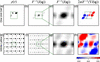Figure 2
Functions calculated from an isolated unit cell of a toy molecule (top row) and from an infinite crystal of the same unit cell (bottom row). The dashed boxes represent the size of the unit cell. (a, e) Electron density; (b, f) autocorrelation function; (c, g) the lowest-order Wigner–Seitz cell of the autocorrelation function (i.e. centered on the origin); (d, h) inverse Fourier transform of the intensity gradients in the horizontal direction, shown within the lowest-order Wigner–Seitz cell. The color scale of the coordinate $[\Delta{\bf r}]$ is indicated below (h).

The purpose of this work is to close the gap between the theoretical magnitude-and-gradient phase retrieval framework proposed by Elser and its application to realistic nanocrystal diffraction data. To this end, we first investigate how molecular-transform intensity gradients could be reliably extracted from nanocrystal diffraction patterns. Using simulated data, we then incorporate these gradients into an iterative reconstruction algorithm and compare its performance directly against a similar iterative algorithm that relies solely on Bragg intensities.

By evaluating both the magnitude-and-gradient and magnitude-only algorithms on simulated datasets covering a wide range of solvent fractions, we assess how gradient information improves reconstruction quality, particularly in regimes where conventional IPR algorithms fail. We further probe the algorithm's robustness under experimentally relevant complications, such as Poisson noise and missing low-resolution data caused by a beamstop. Through these studies, we aim to establish the practical feasibility of magnitude-and-gradient phase retrieval and to clarify under what conditions it can substantially expand the applicability of direct phasing for nanocrystal diffraction.

2. Measuring molecular intensity gradients

Before describing the algorithm, we outline a method for extracting intensity gradients from crystal diffraction patterns. A protein crystal may be described as the convolution $[(\star)]$ of the unit-cell density with a lattice. The following gradient retrieval procedure only applies to crystals with a single molecule per unit cell, so that the asymmetric unit is the whole molecule and the only crystallographic symmetry is translational. Extending this treatment to other space groups remains an important open question. The lattice is, in turn, given by the product of an infinite lattice and the crystal shape function. The real-space crystal density $[\rho_{\rm {cryst}}({\bf r})]$ can thus be written as

$[\rho_{\rm {cryst}}({\bf r}) = \rho_{\rm {mol}}({\bf r})\star[l_{\infty}({\bf r})\ s({\bf r})],\eqno(4)]$

where $[\rho_{\rm {mol}}({\bf r})]$ is the electron density of the repeating unit (e.g. an individual molecule), $[l_{\infty}({\bf r})]$ is an infinite periodic lattice of delta functions at each lattice point and $[s({\bf r})]$ is the lattice shape function, which is one inside the crystal and zero outside. For notation used in the article see Table 1. The measured coherent diffraction $[I_{\rm {cryst}}({\bf q})]$ is proportional to the squared modulus of the Fourier transform of $[\rho_{\rm {cryst}}({\bf r})]$ ,

$[I_{\rm {cryst}}({\bf q}) = |F_{\rm {cryst}}({\bf q})|^{2} = |F_{\rm {mol} }({\bf q})|^{2}\ \left |[L_{\infty}({\bf q})\star S({\bf q})]\right |^{2},\eqno(5)]$

where $[L_{\infty}({\bf q})]$ is the reciprocal lattice, like its real-space counterpart an infinite grid of delta functions, and the `lattice shape transform' $[S({\bf q})]$ is the Fourier transform of $[s({\bf r})]$ . As shown in equation (5) and illustrated in Fig. 3, $[S({\bf q})]$ is replicated at each reciprocal-lattice point, and all peaks are modulated by the molecular structure factors. The width of a Bragg peak, the finest feature in reciprocal space, is inversely proportional to the longest correlation length in the crystal (Ayyer et al., 2018 ). Small crystals therefore exhibit broad Bragg peaks. For large crystals, the spatial coherence of the beam may not be as large as the entire crystal, or the real-space lattice might maintain its correlation only over sub-volumes of the crystal, as in a mosaic crystal. $[S({\bf q})]$ represents the Fourier transform of the coherent volume of the crystal and, in the aforementioned examples, Bragg peaks may thus be significantly wider than one would expect from the crystal size alone.

Table 1
Definition of variables and notation, organized so that quantities defined in both real and reciprocal space appear on the same row

Subscripts denote the object they describe: mol (molecule/asymmetric unit), uc (unit cell), cryst (finite crystal), $[\infty]$ (infinite lattice) and finite (finite lattice).

Real space	Fourier transform	Intensity	Description
Diffraction objects (paired by space)
$[\rho_{\rm {mol}}({\bf r})]$	$[F_{\rm {mol}}({\bf q})]$	$[I_{\rm {mol}}({\bf q}) = \|F_{\rm {mol}}({\bf q})\|^{2}]$	Single molecule/asymmetric unit: the repeating unit and the reconstruction target
$[\rho_{\rm {uc}}({\bf r}^{\rm {uc}})]$	$[F_{\rm {uc}}({\bf q})]$	—	Periodic unit-cell density (formerly $[\rho_{\rm u}]$ ); equals $[\rho_{\rm {mol}}]$ wrapped into the cell
$[\rho_{\rm {cryst}}({\bf r})]$	$[F_{\rm {cryst}}({\bf q})]$	$[I_{\rm {cryst}}({\bf q}) = \|F_{\rm {cryst}}({\bf q})\|^{2}]$	Finite (simulated) crystal (formerly c, C)
$[l_{\infty}({\bf r})]$	$[L_{\infty}({\bf q})]$	$[\|L_{\infty}^{2}({\bf q})\|]$	Infinite lattice of delta functions
$[l_{\rm {finite}}({\bf r})]$	$[L_{\rm {finite}}({\bf q})]$	$[\|L_{\rm {finite}}({\bf q})\|^{2}]$	Finite lattice, $[l_{\rm {finite}} = l_{\infty} s]$ , $[L_{\rm {finite}} = L_{\infty}\star S]$
$[s({\bf r})]$	$[S({\bf q})]$	$[\|S({\bf q})\|^{2}]$	Lattice shape function (1 inside, 0 outside) and lattice shape transform
$[R_{j}({\bf r}) = 2\pi i\,u_{j}\,\rho_{\rm {mol}}]$	$[\nabla_{j}F_{\rm {mol}}({\bf q})]$	$[\nabla_{j}I({\bf q})]$	Gradient replica for axis j; $[{\cal F}\{R_{j}\} = \nabla_{j}F_{\rm {mol}}]$
$[A_{\rm {mol}}(\Delta{\bf r})]$	–	$[I_{\rm {mol}}({\bf q})]$	Continuous autocorrelation of $[\rho_{\rm {mol}}]$ ; $[{\cal F}\{A_{\rm {mol}}\} = I_{\rm {mol}}]$
$[P(\Delta{\bf r})]$	–	$[I({\bf q}_{hk\ell})]$	Patterson function (autocorrelation aliased to the unit cell)

Coordinates and indices		Algorithm and metrics
$[{\bf r}]$	General spatial coordinate	$[\rho_{\rm {mol}}^{(k)},\ z^{(k)}]$	Density iterate and ADMM dual variable at step n (counter unified to n)
$[{\bf r}^{\rm {uc}}]$	Fractional unit-cell coordinate	α	ADMM relaxation/step-size parameter
$[\Delta{\bf r}]$	Interpoint (pair-correlation) distance	σ	Intensity gradient scaling hyperparameter in the Fourier projection
$[{\bf u}({\bf r})]$	Unwrapping function mapping unit-cell to molecular coordinates	$[P_{\rm F,{mag}},\ P_{\rm {O,mag}}]$	Fourier and object projections, magnitude-only algorithm
$[{\bf q}]$	Reciprocal-space coordinate	$[P_{\rm F,{grad}},\ P_{\rm O,{grad}}]$	Fourier and object projections, magnitude-and-gradient algorithm
$[{\bf q}_{hk\ell},\ {\bf q}_{\rm {frac}}]$	Bragg peak position and fractional offset from the nearest peak	$[q_{\rm {stop}}]$	Radius of the central beamstop mask in reciprocal space
j	Spatial dimension index ( x,y,z)	η	Global signal-to-noise ratio parameter
		$[{\cal S}]$	High-resolution shell used for signal normalization
		$[I_{\rm {true}}({\bf q}),\ I_{\rm {noisy}}({\bf q})]$	Noiseless and noisy intensities
		CC	Maximum voxel-wise cross-correlation coefficient
Defining relations: $[\rho_{\rm {cryst}}]$ = $[ \rho_{\rm {mol}}\star(l_{\infty}s)\ \buildrel{\cal F}\over\rightarrow\ F_{\rm {cryst}}]$ = $[F_{\rm {mol}} L_{\rm {finite}}]$ , $[ I _{\rm {cryst}}]$ = $[ I_{\rm {mol}}\,\|L_{\rm {finite}}\|^{2}]$ ; $[\rho_{\rm {mol}}[{\bf u}({\bf r}^{\rm {uc}})]]$ = $[\rho_{ \rm {uc}}({\bf r}^{\rm {uc}})]$ , $[F_{\rm {mol}}({\bf q}_{hk\ell})]$ = $[F_{\rm {uc}}({\bf q}_{hk\ell})]$ ; $[{\cal F}^{-1}\{I_{\rm {mol}}\}]$ = $[A_{\rm {mol}}]$ , $[{\cal F}^{-1}\{ \nabla_{j}I\}]$ = $[-2\pi i\,\Delta r_{j}\,A_{\rm {mol}}]$ .

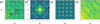Figure 3
(a) Section of a noise-free diffraction pattern with Bragg peaks, i.e. $[I_{\rm {cryst}}({\bf q}_{hk\ell})]$ . $[{\bf q}_{hk\ell}]$ indicates the positions of the Bragg peaks and $[{\bf q}_{\rm {frac}}]$ indicates the fractional offset from the nearest Bragg peak. (b) The lattice shape transform, representing the average intensity relative to the nearest Bragg peak, i.e. $[|S^{2}({\bf q})|]$ . (c) The intensity of the finite lattice transform, i.e. $[|L_{\rm {finite}}^{2}({\bf q})|]$ . (d) Following Spence et al. (2011

), equation (5)

is rearranged to solve for the molecular intensity $[I_{\rm {mol}}({\bf q}) = {I_{\rm {cryst}}({\bf q})}/{|L_{\rm {finite}}^ {2}({\bf q})|}]$ . All intensity scales are presented on a logarithmic scale.

If the band-limited function $[|F_{\rm {mol}}({\bf q})|^{2}]$ varies slowly over each reciprocal-lattice peak, equation (5) indicates that the shape of each peak is approximately identical. Although $[S({\bf q})]$ generally extends to reciprocal distances beyond the spacing between reciprocal-lattice points, the convolution $[L_{\infty}({\bf q})\ \star]$ $[S({\bf q}) = L_{\rm {finite}}({\bf q})]$ is a periodic function that can be fully described over the Brillouin zone of the reciprocal lattice, addressed by the coordinate $[{\bf q}_{\rm {frac}}]$ . Any position in reciprocal space can be expressed as $[{\bf q} = {\bf q}_{hk\ell}+{\bf q}_{\rm {frac}}]$ with $[\forall{\bf q}_{hk\ell}\in]$ $[{\bf q}:L_{\infty}({\bf q})\neq 0]$ and $[-0.5\,\lt\,{\bf q}_{\rm {frac}}\cdot{\bf a}\leq 0.5]$ , where $[{\bf a}]$ is the unit-cell basis.

There are several consequences to this approach. First of all, each crystal will have its own lattice shape transform. Spence et al. (2011) showed that with a sufficiently large ensemble equation (5) holds, with $[S({\bf q})]$ replaced by the average lattice shape transform of the ensemble. Second, compared with conventional data collection strategies, the extraction of intensity gradients at the Bragg peaks requires a significantly finer sampling of intensities throughout the volume of reciprocal space.

The most significant limitation is that all effects of the shape function have to affect the lattice only and leave the unit cell unchanged. If there are symmetries other than translation (i.e. a non-P1 space group), this is broken. Furthermore, surface effects, such as a disordered solvent shell, and strain may also affect the unit cell in unpredictable ways. Disentangling the molecular transform from the lattice shape transform, as described above, is only possible if the unit cell is not distorted, and if there is only one copy of the asymmetric unit in the unit cell.

With this out of the way, we generalize these cases by expressing the merged photon counts (or intensities) of equation (5) as

$[I_{\rm {cryst}}({\bf q}) = I_{\rm {mol}}({\bf q})\ |L_{\rm {finite}} ^{2}({\bf q})|,\eqno(6)]$

with data represented on a fine 3D array. Estimates of $[I_{\rm {mol}}({\bf q}_{hk\ell}) = |F_{\rm {mol}}({\bf q}_{hk\ell})|^{2}]$ can be obtained by integrating the counts in the volume of each peak, normalizing by the integral of $[L_{\rm {finite}}^{2}({\bf q}_{\rm {frac}})]$ , while gradients $[\nabla I_{\rm {mol}}({\bf q}_{hk\ell})]$ can be obtained from the finely sampled intensities $[I_{\rm {cryst}}({\bf q})]$ by first dividing these by $[L_{\rm {finite}}^{2}({\bf q}_{\rm {frac}})]$ to obtain precise estimates of $[I_{\rm {mol}}({\bf q})]$ in the neighborhoods of the Bragg peaks. These steps, however, require a precise estimation of $[L_{\rm {finite}}^{2}({\bf q}_{\rm {frac}})]$ . Following Spence et al. (2011), $[L_{\rm {finite}}^{2}({\bf q}_{\rm {frac}})]$ can be determined by averaging $[I_{\rm {cryst}}({\bf q}_{\rm {frac}})]$ over all Bragg peaks $[{\bf q}_{hk\ell}]$ to give $[\langle I_{\rm {mol}}\rangle\,|S({\bf q}_{\rm {frac}})|^{2}]$ . After normalization, this is convolved with the reciprocal lattice to obtain the periodic $[L_{\rm {finite}}^{2}({\bf q})]$ . The precise estimates of $[I_{\rm {mol}}({\bf q})]$ are thus obtained within the peaks where $[S^{2}({\bf q})]$ is significantly nonzero. For each Bragg reflection, we fit the local intensity distribution along the three reciprocal axes q_x, q_y, q_z; the slopes of these fits yield the three components of $[\nabla I_{\rm {mol}}({\bf q})]$ .

This is easiest when the unit cell is orthogonal, so that the reciprocal axes are orthogonal and the measured intensities fall on an orthogonal sampling grid. This is the case treated in our simulations (Section 4). In general, however, the cell is not orthogonal and the reciprocal axes no longer coincide with the sampling grid. Two approaches are then possible. One can resample the measured intensities onto an orthogonal grid by an affine transformation, rotation and scaling, which aligns the reciprocal axes with the sampling directions (Meisburger et al., 2020 ). Alternatively, one can fit the local intensity distribution along the non-orthogonal reciprocal axes directly, in the measured frame. The latter requires a more involved fit but avoids interpolating the entire dataset, and the associated interpolation errors, incurred by the former.

3. Algorithmic implementation

In this section, we describe the numerical implementation of the proposed phase retrieval framework, which incorporates both Bragg intensities and their local gradients. Building on the formalism introduced in the previous sections, we first define the unwrapping function required to relate the unit-cell density to the molecular density. We then formulate the reciprocal-space constraints arising from both intensity and gradient measurements, followed by the corresponding projection operators. Real-space constraints, including support and positivity, are subsequently introduced and combined within a divide-and-concur framework. Finally, we present the iterative projection scheme used to solve the resulting constrained optimization problem and outline the specific implementation details used in our simulations.

3.1. The unwrapping function

As seen in equation (5), $[F_{\rm {cryst}}({\bf q})]$ is composed of the multiplication of $[L_{\rm {finite}}({\bf q})]$ and $[F_{\rm {mol}}({\bf q}) = {\cal F}\{\rho_{\rm {mol}}({\bf r})\}]$ . We aim to form a Fourier synthesis of the molecular density $[\rho_{\rm {mol}}({\bf r})]$ . For crystallography based on Bragg intensities alone, one performs this synthesis only at the reciprocal-lattice points from $[F_{\rm uc}({\bf q}_{hk\ell}) = {\cal F}\{\rho_{\rm {cryst}}({\bf r}^{{\rm uc}})\}]$ , to recover the unit cell of the periodic density $[\rho_{\rm {cryst}}({\bf r}^{\rm {uc}})]$ of equation (4) within the primitive unit cell. This unit cell is a parallelepiped containing the asymmetric unit. The choice of the origin of this unit cell is arbitrary and only modifies $[F_{\rm uc}({\bf q}_{hk\ell})]$ by a phase ramp, even if the boundaries of the unit cell may slice across the molecule.

The electron density of the unit cell $[\rho_{\rm {uc}}({\bf r}^{\rm {uc}})]$ is not the same as that of the molecular unit $[\rho_{\rm {mol}}({\bf r})]$ , which is the single molecule that is repeated at each lattice position to form the crystal. It is important to distinguish between these two quantities: the unit-cell density is a periodic representation constrained by the computational domain, whereas the molecular density corresponds to the physical object of interest. While the two objects share $[F_{\rm uc}({\bf q}_{hk\ell}) = F_{\rm {mol}}({\bf q}_{hk\ell})]$ , as seen from equation (4) and equation (5), away from the reciprocal-lattice points (including infinitesimally close to them as needed to define a gradient) they differ. Here, the diffraction intensities depend on the physical structure of the crystal and particularly on how the crystal is terminated (Kirian et al., 2015). One way to appreciate this difference is that the crystal density $[\rho_{\rm {cryst}}({\bf r})]$ in equation (4) is not defined as an infinite crystal multiplied by a shape $[s({\bf r})]$ , whose transform would correspond to that of the infinite crystal convolved with the lattice shape transform. In that case, the molecules on the surfaces of the crystal might be truncated by the arbitrary boundaries of the unit cell, which is unphysical. Equation (4) shows instead that the entirety of the crystal is given by the compact structure $[\rho_{\rm {mol}}({\bf r})]$ repeated at a finite number of lattice positions. The surface of the crystal in that case consists of whole molecules.

Many crystals contain more than one molecule or asymmetric unit per unit cell. For such crystals, it is likely that their termination behavior is not regular, meaning that the crystal may terminate in partial unit cells. For example, a 1D crystal with unit cell `ab' could start and end with `a' (`ababa" rather than `ababab'). As a result, the measured intensities average over cells with different terminations, so that the finite crystal presents several distinct effective transforms rather than the single transform of a fully periodic crystal (Kirian et al., 2015). There has been work to create algorithms that incorporate and estimate such irregular terminations (Chen et al., 2023). As stated above, the gradient calculation is restricted to a single molecular unit.

Because IPR algorithms are executed using the discrete Fourier transform, it is practically necessary to reconstruct the density within a strictly periodic volume, such as the unit cell. To obtain $[F_{\rm {mol}}({\bf q})]$ from $[F_{\rm uc}({\bf q})]$ , following Elser (2013), the unit-cell density can be expressed as

$[\rho_{\rm {mol}}[{\bf u}({\bf r}^{\rm {uc}})] = \rho_{\rm {uc}}( {\bf r}^{\rm {uc}}).\eqno(7)]$

Here the `unwrapping function' $[{\bf u}({\bf r})]$ maps the fractional coordinate $[{\bf r}^{\rm {uc}}]$ within the unit cell to positions within the single asymmetric unit, which may extend beyond the boundary of the unit cell. Consequently, expressing $[F_{\rm {mol}}({\bf q})]$ in unit-cell coordinates (Elser, 2013) yields

$[F_{\rm {mol}}({\bf q}) = \int\rho_{\rm {uc}}({\bf r}^{\rm {uc}})\exp[2 \pi i{\bf u}({\bf r}^{\rm {uc}})\cdot{\bf q}]\,{\rm d}{\bf r}^ {\rm {uc}}.\eqno(8)]$

The choice of $[{\bf u}({\bf r})]$ is not unique, since some $[{\bf r}]$ can map to multiple $[\rho_{\rm {mol}}({\bf r})]$ , and the boundary between molecular units can be chosen to lie anywhere within the solvent region. The wrapping of the asymmetric unit in the unit cell is illustrated in Fig. 4. A portion of a 2D crystal is depicted in Fig. 4(a), showing several repeated molecules. Lattice positions, $[l_{\infty}({\bf r})]$ , and the corresponding unit cell are indicated. The origin of the lattice and the unit cell is arbitrary. Because IPR is performed on a periodic computational grid, the reconstruction naturally yields a unit-cell density rather than the molecular density. To recover the underlying molecular density, it is therefore necessary to account for the wrapping of the molecule across unit-cell boundaries. The x and y components of the unwrapping function are shown in Figs. 4(b) and 4(e). These map the fractional coordinates of the unit cell to the single molecule and ensure that the Fourier integral of equation (8), made over the domain of the unit cell, is equal to that of the single molecule.

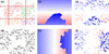Figure 4
(a) Slice through a protein crystal, with unit-cell boundaries shown in red and each distinct protein shown in a different color. (d) Slice through a single unit cell, i.e. in the space $[\rho_{\rm {mol}}]$ ( $[{\bf r}]$ ). (b), (e) The unwrapping functions $[{\bf u}_{x}({\bf r})]$ and $[{\bf u}_{y}({\bf r})]$ (red: positive; blue: negative; white: zero). Although the protein is cut off along both x and y, this slice only shows the effect along y. (c), (f) Slices through the replicas $[{\bf R}_{x}({\bf r})]$ and $[{\bf R}_{y}({\bf r})]$ . Each component of $[{\bf u}({\bf r})]$ marks transitions only along its respective axis.

3.2. Reciprocal-space constraints

The phasing algorithm of Elser (2013) makes use of four sets of Fourier constraints: the Fourier magnitudes obtained from the square root of the Bragg intensities $[I_{\rm {mol}}({\bf q}_{hk\ell})]$ , and the three components of the gradients of the intensities at reciprocal-lattice vectors $[{\bf q}_{hk\ell}]$ . Since the following analysis focuses exclusively on intensities and gradients evaluated at the reciprocal-lattice points ( $[{\bf q} = {\bf q}_{hk\ell}]$ with $[{\bf q}_{\rm {frac}} = 0]$ ), we drop the `mol' and ` hkl' subscripts for the sake of brevity. Furthermore, as established previously, our analysis focuses solely on the gradients of $[F_{\rm {mol}}]$ and $[F_{\rm {mol}}({\bf q}_{hk\ell}) = F_{\rm uc}({\bf q}_{hk\ell})]$ ; for notational convenience, we hereafter refer to it simply as F.

The modulus constraint from the intensities is straightforward. The modulus of the Fourier transform of the density should equal the square root of the diffraction intensities:

$[|{\cal F}\{\rho({\bf r}^{\rm {uc}})\}| = |F({\bf q})| = \sqrt{I({\bf q})}.\eqno(9)]$

By applying the chain rule, the gradients of the intensities can be expanded as

$[\nabla_{j}I({\bf q}) = \nabla_{j}|F({\bf q})|^{2} = 2\,{\rm Re}[{F^{*}({\bf q})}\nabla_{j}F({\bf q})]\eqno(10)]$

for each dimension $[j\in\{x,y,z\}]$ . From equation (8), it follows that

$[\eqalignno{\nabla_{j}F({\bf q})& = \nabla_{j}\int\rho({\bf r}^{\rm {uc}})\exp[2\pi i{\bf u}({\bf r}^{ \rm {uc}})\cdot{\bf q}]\,{\rm d}{\bf r}^{\rm {uc}}&\cr & = 2\pi i\int{\bf u}_{j}({\bf r}^{\rm {uc}})\,\rho({\bf r}^{\rm {uc}})\,\exp[2\pi i{\bf u}({\bf r}^{\rm {uc}})\cdot{\bf q}] \,{\rm d}{\bf r}^{\rm {uc}}.&(11)}]$

Substituting this result into equation (10) yields the constraint relating the Fourier transform and its gradients,

$[2{\rm Re}[{\cal F}\{\rho({\bf r})\}^{*}\,{\cal F}\{{\bf R}_{j}({\bf r})\}] = \nabla_{j}I({\bf q}),\eqno(12)]$

where, from equation (11),

$[{\bf R}_{j}({\bf r}^{\rm {uc}}) = 2\pi i\,{\bf u}_{j}({\bf r}^{ \rm {uc}})\rho({\bf r}^{\rm {uc}})\eqno(13)]$

are the three real-space versions of the electron density, each multiplied by the unwrapped coordinate along j, $[{\bf u}_{j}({\bf r}^{\rm {uc}})]$ . Examples of this are shown in Fig. 4. Note that a change in the choice of the origin of the unit cell leads to a non-trivial change of $[\nabla F({\bf q})]$ but, as seen from equation (3), this has no effect on the calculation of $[\nabla|F({\bf q})|^{2}]$ .

3.3. Fourier-space projection

In the Results section, we will discuss and compare two algorithms which differ only in the projections they use. Here, we present one variant that relies on gradient information, which we refer to as the magnitude-and-gradient algorithm, with the corresponding projection denoted $[P_{\rm grad}]$ . The other does not use this information and is called the magnitude-only algorithm with the corresponding projections being denoted $[P_{\rm mag}]$ . For readability and convenience, we drop the explicit $[{\bf r}]$ and $[{\bf q}]$ dependence in the projection definitions for the rest of this subsection.

First, we define the magnitude-only case. While we defined ρ and F as the electron density and its Fourier transform, respectively, in the following, we use $[\rho^{(k)}]$ and F^(k) to denote the input of a projection and $[\rho^{(k+1)}]$ and F^(k+1) for the output of a projection. So, considering only equation (9), the Fourier projection $[P_{{\rm F,mag}}]$ simply updates the estimate by replacing the calculated amplitudes with the measured ones, $[\sqrt{I}]$ .

Magnitude-only Fourier projection P_F,mag

Mapping F^(k) to F^(k+1) on the constraint equation (9), the projection updates the estimate such that

$[\tilde{P}_{\rm F,{mag}}:F^{(k+1)} = \sqrt{I}{{F^{(k)}} \over {|F^{(k)}|}}.\eqno(14)]$

Here, the phase $[\varphi = \arg(F_{k})]$ remains unchanged, while the amplitude is constrained to match the experimental data. If we want to express the projection in real space, mapping from $[\rho^{(k)}]$ to $[\rho^{(k+1)}]$ , we can use the Fourier transform $[{\cal F}]$ and its inverse $[{\cal F}^{-1}]$ to write

$[P_{\rm F,{mag}}:\rho^{(k+1)} = {\cal F}^{-1}\left\{\tilde{P}_{{\rm F,mag}}\left[{\cal F }\left(\rho^{(k)}\right)\right]\right\}.\eqno(15)]$

As mentioned in the Introduction, the divide-and-concur method (Gravel & Elser, 2008) can be used to apply iterative projection algorithms to more than two sets of constraints. Here, four copies of the electron density are concatenated into one long state vector $[{\boldrho}]$ . In the divide projection each of the four constraint projections, corresponding to the modulus constraint of equation (9) and the three gradient constraints of equation (12), are applied to a different replica within $[{\boldrho}]$ . The concur projection then enforces agreement between the various projections by averaging all replicas into a single estimate of the electron density. Following Elser (2013), $[{\boldrho}]$ is defined not as four equivalent copies of the electron-density estimate ρ but with the coordinate-weighted versions of equation (13) as $[{\boldrho} = (\rho,R_{x},R_{y},R_{z})]$ , where the other replicas are determined by $[{\bf R} = {\bf u}\rho]$ [i.e. equation (13)]. The main benefit is that the Fourier transform of $[{\boldrho}]$ is then equal to the four quantities for which constraints exist, namely $[{\bf F} =]$ $[(F,\nabla_{x}F,\nabla_{y}F,\nabla_{z}F)]$ , by applying the Fourier transforms as defined in equation (8) and equation (11). To incorporate the gradient constraints into the Fourier or `data' projection, we follow the approach of Elser (2013). We refer the reader to Appendix A for its derivation.

The gradient-augmented Fourier projection enables the reconstruction of electron density by satisfying four independent constraints per Bragg peak: one for the measured intensity and three for the components of the molecular intensity gradient. To jointly satisfy these constraints, the algorithm minimizes the L2 distance between the input configuration $[{\bf F}^{(k)}]$ and the projected output $[{\bf F}^{(k+1)}]$ . The process begins by finding the minimum distance to reach the constraint using the method of Lagrange multipliers, which corrects the input gradient estimates along the direction of the structure factor. The stationarity condition of the Lagrangian yields an expression for the distance between the input and output configurations. This can be written as a non-convex trigonometric potential, specifically a double-angle cosine function of an unknown phase. By identifying the global minimum of this potential, the algorithm determines an optimal phase that simultaneously satisfies the magnitude constraint and aligns with the observed peak shifts, effectively turning an underdetermined system into an overdetermined one that is more resilient to noise.

Magnitude-and-gradient Fourier projection P_F,grad

To map $[{\bf F}^{(k)}]$ to $[{\bf F}^{(k+1)}]$ satisfying the constraint set given by equation (9) and equation (12), we update the Fourier transform and its gradients according to

$[\tilde{P}_{{\rm F,grad}}:\left\{\matrix{F^{(k+1)}\hfill& = \sqrt{I}\exp(i\varphi), \hfill\cr (\nabla_{j}F)^{(k+1)}& = (\nabla_{j}F)^{(k)}-2\pi F^{(k+1)}\lambda_{j}. }\right.\eqno(16)]$

Note that one first calculates F^(k+1), where the phases φ are updated to reflect information from both F^(k) and $[(\nabla F)^{(k)}]$ . To then obtain $[\nabla F^{(k+1)}]$ , one also needs to find the Lagrange multiplier $[\lambda_{j}]$ . This projection was derived by Elser (2013). Appendix A provides the derivation of $[\lambda_{j}]$ and φ [equations (30) and (39), respectively].

To map from $[{\boldrho}^{(k)}]$ to $[{\boldrho}^{(k+1)}]$ we thus define $[P_{{\rm F,grad}}]$ like $[P_{{\rm F,mag}}]$ . First, one applies the Fourier transform $[{\cal F}]$ to each of the four replicas in $[{\boldrho}^{(k)}]$ to obtain $[{\bf F}^{(k)}]$ . Then, one inserts the result into $[\tilde{P}_{{\rm F,grad}}]$ to obtain the updated F^(k+1) and $[(\nabla_{j}F)^{(k+1)}]$ . Lastly, the inverse Fourier transform $[{\cal F}^{-1}]$ is applied to $[{\bf F}^{(k+1)}]$ to obtain the updated replicas in real space $[{\boldrho}^{(k+1)}]$ .

3.4. Real-space constraints and projections

In real space, we enforce a total of three constraints. We discuss first the constraints used for the magnitude-only and magnitude-and-gradient algorithms and then how these fit into the divide-and-concur framework of the magnitude-and-gradient algorithm. The first is the positivity constraint, which reflects the physical requirement that electron densities cannot be negative. This is expressed as

$[\forall{\bf r}:\rho({\bf r})\geq 0.\eqno(17)]$

Second, structural information is confined within a finite support γ. Outside this region, the density is assumed to be a uniform solvent, $[\rho_{\rm {solvent}}]$ ,

$[\forall{\bf r}\ \notin\ \gamma:\rho({\bf r}) = \rho_{\rm {solvent}}.\eqno(18)]$

In practice, the exact support is rarely known a priori. To address this, we employ a `shrinkwrap' algorithm (Marchesini et al., 2003 ), which dynamically updates the support during the reconstruction. It begins with a loose initial estimate, often the entire unit cell, and iteratively wraps more tightly around the object as the density estimate improves (we describe our implementation in Section 3.5).

Combining the positivity [equation (17)] and support [equation (18)] constraints yields the real-space projection for the magnitude-only algorithm:

Real-space object projection P_O,mag

Applying the combined support and positivity constraints to the current estimate $[\rho^{(k)}]$ yields the updated estimate $[\rho^{(k+1)}]$ :

$[P_{{\rm O,mag}}:\left\{\matrix{\rho^{(k+1)}({\bf r}) = \rho^{(k)}({\bf r})& {\rm if }\ \rho^{(k)}\in\ {\rm support\ and }\ \rho^{(k)}\geq 0,\cr \rho^{(k+1)}({\bf r}) = 0\hfill &{\rm else }.\hfill}\right.\eqno(19)]$

As discussed previously, the magnitude-and-gradient Fourier projection generates four independent estimates within the state vector $[{\boldrho}({\bf r})]$ . Within the divide-and-concur framework, the generation of these independent estimates constitutes the `divide' step. To complete the operation, the real-space `concur' projection must reconcile these independent replicas to yield a single, coherent density estimate, $[\rho({\bf r})]$ , at each position $[{\bf r}]$ . This reconciliation enforces internal consistency between the replicas but does not impose physical constraints on the density. For readability, we hereafter drop the explicit spatial dependence $[({\bf r})]$ from our notation. Because the gradient replicas are inherently tied to the density through the relationship $[{\bf R}_{j} = 2\pi i{\bf u}_{j}\rho]$ , we must formulate a joint estimate that forces the replicas to concur by satisfying this structural coupling. To accomplish this, Elser (2013) proposed a distance-minimizing projection, which maps the input state vector $[{\boldrho}^{(k)}]$ to a unified density $[\bar\rho]$ :

$[P_{\rm reconcile}:\bar\rho = {\rm Re}\left[{{\rho^{(k)}+\sum_ {j}{\bf u}_{j}\cdot{\bf R}_{j}^{(k)}/2\pi i} \over {1+\sum_{j}{\bf u}_{j} \cdot{\bf u}_{j}}}\right].\eqno(20)]$

This projection effectively computes a weighted average of the four replicas, where the gradient contributions are weighted by their distance from the origin.

Regardless of whether we use the magnitude-only or magnitude-and-gradient algorithm, the real-space constraints must also be satisfied. We thus include these as a side constraint and apply this projection after having reconciled the four different replicas in $[\bar\rho]$ , yielding the final updated density $[\rho^{(k+1)}]$ . From this constrained density, we then cast the consistent gradient replicas $[{\bf R}_{j}^{(k+1)}]$ using equation (13). The complete real-space projection for the magnitude-and-gradient algorithm, denoted as $[P_{{\rm O,grad}}]$ , is summarized below.

Magnitude-and-gradient object projection P_O,grad

To apply $[P_{{\rm O,grad}}]$ from $[{\boldrho}^{(k)}]$ to $[{\boldrho}^{(k+1)}]$ , we perform the following steps:

(i) Apply the reconciliation projection $[\bar\rho = P_{\rm reconcile}[{\boldrho}^{(k)}]]$ to reconcile the four independent replicas into a single density estimate.

(ii) Apply the real-space constraints $[\rho^{(k+1)} = P_{{\rm O,mag}}(\bar\rho)]$ (positivity and support) to obtain the constrained object $[\rho^{(k+1)}]$ .

(iii) Cast the updated object $[\rho^{(k+1)}]$ back into the gradient replicas using the relationship $[{\bf R}_{j}^{(k+1)} = 2\pi i\,{\bf u}_{j}\rho^{(k+1)}]$ for each j, yielding the fully updated state vector [ $[\rho^{(k+1)}]$ , $[{\bf R}_{x}^{(k+1)},{\bf R}_{y}^{(k+1)},{\bf R}_{z}^{(k +1)}]$ ].

3.5. Iterative projection algorithm

After defining the relevant projections, we will now present the iterative projection framework, which we use for both the magnitude-only and magnitude-and-gradient algorithms. It is based on the alternating direction method of multipliers (Boyd et al., 2011 ), which is similar but not identical to the version Elser (2013) used in their original publication and is given by

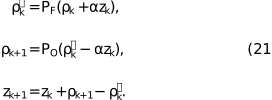
$[\eqalign{\rho_{k}^{\prime}& = P_{\rm F}(\rho_{k}+\alpha z_{k}),&\cr \rho_{k+1}& = P_{\rm O}(\rho_{k}^{\prime}-\alpha z_{k}),&\cr z_{k+1}& = z_{k}+\rho_{k+1}-\rho_{k}^{\prime}.}\eqno(21)]$

Here α acts as a relaxation or step-size parameter that controls the update of the discrepancy variable z_k. Empirical testing showed that values of α between 0.5 and 0.8 yielded comparable convergence stability. A weight of $[\alpha = 0]$ reduces to the error reduction algorithm, whereas a weight of 1 gives the Douglas–Rachford algorithm (Elser, 2013). For initial values, we set the first real-space guess $[\rho_{0}({\bf r})]$ to the Fourier transform of $[\sqrt{I}]$ with random phases and set $[z_{0}({\bf r}) = 0]$ .

The magnitude-only algorithm uses $[P_{{\rm O,mag}}]$ and $[P_{{\rm F,mag}}]$ , whereas the magnitude-and-gradient algorithm uses $[P_{{\rm O,grad}}]$ and $[P_{{\rm F,grad}}]$ .

In experiments, the unwrapping function $[{\bf u}({\bf r})]$ is not known before reconstruction. But, as shown by Elser (2013), the reconstruction results are only weakly affected by iteratively estimating $[{\bf u}({\bf r})]$ during reconstruction. Therefore, we do not estimate $[{\bf u}({\bf r})]$ in our simulations but instead use a ground-truth unwrapping function for all reconstructions. Also, we use $[\sigma = 3]$ in all experiments, following Elser (2013).

With respect to the support constraint in the real-space projection, several strategies were considered, including fixed and adaptively updated supports (Marchesini et al., 2003). The fixed support can be either the exact support $[\gamma_{\rm true}]$ that matches the molecule, a looser support or a support covering the entire unit cell. For the looser support we Gaussian blurred and thresholded the ground-truth electron density to generate a support which contains the true support as well as some solvent area. This threshold was set as the median pixel value of all $[{\bf r}\ \notin\ \gamma_{\rm true}({\bf r})]$ , such that the solvent region was halved between being inside and outside of the support. In our implementation of the shrinkwrap support, we Gaussian blurred the current iterate and updated the support according to the thresholded blurred estimate every ten steps, starting from a support covering the entire unit cell.

4. Results

4.1. Dependence on solvent fraction

This section evaluates the robustness of the magnitude-and-gradient algorithm, specifically its performance across different solvent fractions and its resilience to significant noise.

All numerical experiments followed a standardized simulation pipeline. The repeating unit $[\rho({\bf r})]$ is represented as a discretized electron-density map on a regular voxel grid. A finite crystal is constructed by placing this unit on a periodic lattice,

$[c({\bf r}) = \sum_{{\bf h}}\rho({\bf r}+{\bf h}\cdot{\bf a}),\eqno(22)]$

where $[{\bf h}\in[0,H]^{d}]$ defines the integer grid coordinates for a crystal of dimension d, and $[{\bf a}]$ denotes the pixel distance between adjacent repeating units (which corresponds to the unit-cell dimensions, unless otherwise stated). This construction yields a crystal of extent $[H{\bf a}]$ containing H^d repeating units. To achieve adequate sampling in reciprocal space, the array is zero-padded by an additional $[(H+1){\bf a}]$ in all dimensions. From the simulated crystal intensities $[I_{\rm {cryst}}]$ , the lattice shape function $[S^{2}({\bf q})]$ is estimated to remove the finite-lattice contribution $[L_{\rm {finite}}^{2}({\bf q})]$ for all accessible Bragg peaks on the simulated grid. This procedure isolates the molecular intensities $[I_{\rm {mol}}({\bf q})]$ and their gradients $[\nabla I_{\rm {mol}}({\bf q})]$ . To ensure statistical robustness, all reconstructions were repeated 25 times per dataset from random phase initializations. Each reconstruction was iterated for 1000 steps, well beyond the typical convergence threshold. The resulting reconstructions were aligned in real space, averaged and compared against the ground-truth electron density $[\rho_{\rm gt}]$ of the repeating unit using the voxel-wise cross-correlation coefficient CC,

$[{\rm CC}[\rho({\bf r}),\rho_{\rm gt}({\bf r})] = {{\sum_{{\bf r }}[\rho({\bf r})-\langle{\rho}({\bf r})\rangle][\rho_{\rm gt}({\bf r})- \langle{\rho}_{\rm gt}({\bf r})\rangle]} \over {\sqrt{\sum_{{\bf r}}[\rho({\bf r })-\langle{\rho}({\bf r})\rangle]^{2}\sum_{{\bf r}}[\rho_{\rm gt}({\bf r})-\langle{\rho}_{\rm gt}({\bf r})\rangle]^{2}}}},\eqno(23)]$

where $[\langle\rho({\bf r})\rangle]$ is the mean over $[{\bf r}]$ , i.e. $[\langle{\rho}({\bf r})\rangle = \sum_{{\bf r}}\rho({\bf r})/\sum_{ {\bf r}}1]$ . The reconstructed density can be shifted by an arbitrary offset as well as inverted through the origin without modifying the calculated diffraction pattern. This ambiguity, however, affects the calculated CC. Accordingly, the CC was evaluated over all translational offsets (with periodic boundaries) and for both the original and mirrored ground truth $[\rho_{\rm gt}(-{\bf r})]$ , and the maximum value was taken as the final CC. A visual summary of these steps can be seen in Fig. S1 in the supporting information.

We first show the effect of the reconstruction process on a 2D example, which facilitates visual inspection. The computational framework is similar to that used for the 3D crystals. The 2D molecular unit, a grayscale test image, was combined with varying levels of zero-padding around the object to simulate different levels of solvent fraction. These padded objects were placed in a $[5\times 5]$ unit-cell grid, which was further padded by zeros to simulate a finite crystal. The corresponding $[I_{\rm {cryst}}]$ and $[\nabla I_{\rm {cryst}}]$ were then computed as described above. In Fig. 5, we show a side-by-side comparison of the magnitude-only and magnitude-and-gradient IPR algorithms at different solvent fractions.

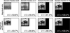Figure 5
Visual comparison of magnitude-only reconstruction and magnitude-and-gradient reconstruction at different solvent fractions, where the black background indicates the simulated solvent. We display the cross-correlation coefficient (CC) between the reconstruction and the ground truth, excluding the solvent area, in the bottom-right corner.

As discussed in the Introduction, a square 2D object of edge length E requires a unit cell of at least $[2E\times 2E]$ to prevent aliasing of its autocorrelation function. Given that the object area is E² and the required unit-cell area is 4E², this theoretical limit inherently dictates a minimum solvent fraction of $[(4E^{2}-E^{2})/4E^{2} = 3/4 = 75\%]$ . Ensuring the autocorrelation function remains unaliased means that all information is maintained. At this limit, the magnitude-only algorithm accurately reconstructs the object.

For solvent fractions between 1/2 and 3/4, the reconstruction quality decreases, yet the object's primary structural features are still preserved. This behavior is explained by the constraint ratio (Elser & Millane, 2008) for the support constraint. For a unit cell with volume $[(\alpha E)^{d}]$ in d dimensions containing only solvent and an object with E^d, there are E^d unknowns, corresponding to the volume of the object. There are $[(\alpha E)^{d}/2]$ independent intensity constraints accounting for the Friedel symmetry of the diffraction pattern for real-valued objects. A solvable system requires a constraint ratio greater than unity:

$[1\,\gt\,{{(\alpha E)^{d}/2} \over {E^{d}}}\rightarrow\alpha\,\gt\,{\root d \of 2}.\eqno(24)]$

This implies that with a support constraint alone one needs more than a solvent fraction of 1/2, consistent with the observed behavior.

Incorporating intensity gradients substantially modifies this balance. The resulting constraint ratio, even in the absence of any solvent ( $[\alpha = 1]$ ), is (1+d)E^d/2E^d. In two dimensions, this increases the number of independent constraints by a factor of three. As a consequence, the resulting constraint ratio is then equal to $[3E^{2}/2E^{2} = 1.5]$ , and so reconstruction is, in principle, feasible for any solvent fraction. Just as in the case of magnitude-only, a constraint ratio only marginally greater than unity was found to be insufficient for a perfect reconstruction. In the absence of solvent, the magnitude-and-gradient algorithm recovered a discernible image, though noticeable artifacts remained. Yet, adding just a small area of solvent, equivalent to a solvent fraction of 17%, improved the reconstruction, achieving a CC above 99%.

Building on this 2D proof of concept, we extended our evaluation to simulated 3D protein structures. We obtained the atomic coordinates from a selection of ten proteins with diverse solvent fractions and unit-cell parameters, all belonging to the P1 space group. An overview of these characteristics, including their PDB identifiers, is provided in Fig. 6 and Table 2. We then generated electron-density maps using the gemmi library (Wojdyr, 2022 ) on a grid with a 0.67 Å spacing.

Table 2
Shorthand names for structures used in this study, including unit-cell parameters and solvent fraction (MW = molecular weight)

Shorthand	Full name	PDB code	Cell volume (nm³)	Solvent fraction
RSV F	Respiratory syncytial virus fusion glycoprotein F	8ydl	336.2	0.636
GH168	Endo-fucanase, glycoside hydrolase family GH168	9f9v	168.6	0.365
SLP	S-layer protein complex	9f8f	405.2	0.545
hCRBPII-R58Y	Human cellular retinol-binding protein II, R58Y mutant	9de1	64.1	0.312
HRP-2	PWWP domain of hepatoma-derived growth factor-related protein 2	9i7a	53.5	0.390
NikK	Periplasmic nickel transporter component NikK	9gcb	99.5	0.334
HBDH	3-Hydroxybutyrate dehydrogenase	9c5m	568.4	0.414
hCRBPII-R58A	Human cellular retinol-binding protein II, R58A mutant	9dfb	64.4	0.389
RCC1	Regulator of chromosome condensation 1	1a12	280.5	0.375
GapN	Non-phosphorylating NADP⁺-dependent glyceraldehyde-3-phosphate dehydrogenase	9raz	858.8	0.303

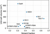Figure 6
Overview of the crystal's solvent fraction, unit-cell size and PDB reference used in the simulations.

For each protein, we constructed a $[5\times 5\times 5]$ unit-cell crystal surrounded by a zero-padded region with a total of six unit-cell lengths along each axis. This specific crystal size represents a computational compromise: it is sufficiently large to produce well defined, broadened Bragg peaks suitable for gradient extraction, while remaining computationally tractable. To explore the limits of the algorithm across a broader range of solvent environments, additional datasets were generated by increasing the space between molecules, resulting in solvent fractions as high as 92%.

Representative slices of two crystals are displayed in Fig. 7: one featuring a realistic solvent fraction of 33% and another where the intermolecular spacing has been artificially increased to probe higher solvent fractions, in this case 80%. The artificially increased solvent crystals were utilized only to compare the performance of the magnitude-and-gradient and magnitude-only algorithms.

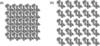Figure 7
A slice through electron densities of protein GapN in a P1 crystal of size $[5\times 5\times 5]$ unit cells. (a) We show a realistic crystal with a solvent fraction of 33%. (b) We show the same molecule but with extra 20% unit-cell lengths of extra solvent between each lattice point, yielding a solvent fraction of 80%. Individual molecular units are displaced to increase intermolecular spacing.

Following the simulation pipeline established for the 2D proof-of-concept study, we generated noise-free diffraction patterns for these 3D crystals. We identified the Bragg peaks and estimated the lattice shape transform to recover both the molecular intensities $[I_{\rm {mol}}({\bf q}_{hk\ell})]$ and their gradients $[\nabla I_{\rm {mol}}({\bf q}_{hk\ell})]$ . A comparison of the algorithms is shown in Fig. 8, where the CC between the reconstruction and ground truth is shown as a function of solvent fraction. The magnitude-and-gradient algorithm reconstructs the structure for all available solvent fractions.

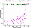Figure 8
Comparison of magnitude-only and magnitude-and-gradient algorithms at different solvent fractions of both real proteins from the PDB and unit cells with increased solvent fraction. Each data point represents the mean CC of the electron density averaged over 25 runs.

The magnitude-only algorithm reliably retrieves the electron density only for solvent fractions exceeding approximately 0.8. Below this limit, the average CC drops sharply, signifying a failure to recover the correct structure. This is consistent with current literature, which notes that state-of-the-art ab initio methods generally require solvent fractions above 0.7 (Kingston & Millane, 2022).

In contrast, and consistent with our 2D observations (Fig. 5), the magnitude-and-gradient algorithm demonstrates a significantly extended operational range. It successfully recovered the correct structure across all tested solvent fractions, maintaining an average CC above 0.97 in all cases. While minor artifacts persist even at high solvent fractions, likely due to an inaccurate gradient estimation step, these results confirm that gradient information effectively supplies the necessary constraints to solve structures of low-solvent crystals.

4.2. Robustness to noise

Next, we evaluated the performance of the magnitude-and-gradient algorithm under conditions that more closely approximate experimental conditions. To this end, we introduced synthetic noise to the diffraction patterns. Because the protein samples exhibit diverse unit-cell parameters and intensity distributions, we define a standardized noise metric to ensure meaningful comparisons across the datasets. For these robustness evaluations, we excluded the artificially inflated solvent cases and focus exclusively on crystals with realistic solvent fractions.

To model the noise, an Anscombe-type approximation was employed (Anscombe, 1948 ), whereby the Poisson distribution is approximated as Gaussian with a standard deviation proportional to the square root of the measured photon counts,

$[I_{\rm {noisy}}({\bf q}) = I_{\rm {true}}({\bf q})+\sqrt{I_{\rm {true}} ({\bf q})}{{\sqrt{\langle I\rangle_{{\cal S}}}} \over {\eta}} {\cal N}(0,1).\eqno(25)]$

Here $[I_{\rm {true}}({\bf q})]$ denotes the calculated noiseless intensity, $[I_{\rm {noisy}}({\bf q})]$ the resulting noisy value and $[{\cal N}(0,1)]$ a standard normal deviate. To facilitate a consistent comparison across protein structures with varying unit-cell parameters and scattering strengths, we normalize the noise magnitude to a characteristic signal level, $[\langle I\rangle_{{\cal S}}]$ . This reference value is calculated as the average intensity of all Bragg reflections within a high-resolution shell $[{\cal S}]$ spanning 1.9 to 2.1 Å. This specific shell is chosen as it is a common resolution limit dictating the feasibility of successful structure determination. By using $[\langle I\rangle_{{\cal S}}]$ as a benchmark, we are able to introduce a global SNR parameter, η, enabling uniform scaling of the noise level across datasets.

The left panel of Fig. 9 visualizes the resulting average SNR at the Bragg peaks as a function of resolution, plotted here for a baseline scenario where the global scaling parameter is set to $[\eta = 1]$ . While the exact SNR curves vary slightly among the ten test proteins due to their differing unit-cell parameters and scattering distributions, they all exhibit the same fundamental behavior: as the resolution increases (smaller d spacing), the measured intensity $[I_{\rm {true}}]$ decreases. Because the noise model dictates that noise scales with the square root of the intensity, the SNR is exceptionally high in the low-resolution shells and decreases with resolution. In the intermediate-resolution shells between 10 and 4 Å, the SNR remains relatively stable at roughly four to 12 times the baseline η. However, in the high-resolution shells beyond the benchmark $[{\cal S}]$ , the effective SNR drops below the nominal η reported here. As defined by equation (25), any modulation of η results in a linear, proportional shift of the entire SNR curve. In Fig. S2, we show a slice through the intensities for for three different noise regimes.

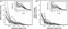Figure 9
(a) Average SNR at Bragg peaks as a function of resolution, calculated by $[I_{\rm {true}}/{\rm std}(|I_{\rm {true}}-I_{\rm {noisy}}|)]$ where std computes the standard deviation. The red dot is the signal strength indicator η, which normalizes the SNR within the resolution shell $[{\cal S}]$ between 1.9 and 2.1 Å – in this case to $[\eta = 1]$ . (b) SNR of the molecular gradients, comparing gradients calculated from $[I_{\rm {true}}]$ and $[I_{\rm {noisy}}]$ . The insets give zoomed-in views of the SNR at the Bragg peaks at high resolution.

Looking at the right panel in Fig. 9, we see that the SNR of the estimated intensity gradients $[\nabla I({\bf q})]$ follows a nearly identical downward trend, with values that are broadly similar but slightly lower than the intensity SNR. This slight reduction occurs because gradient estimation incorporates multiple neighboring points around the averaged lattice shape function $[S^{2}({\bf q})]$ , where intensity values are at most 50% of the Bragg peak maximum. Despite incorporating these lower-intensity neighborhood values, the extracted gradients maintain a relative fidelity of roughly 60% to 70% compared with the raw intensities across the entire resolution range.

In addition to noise, the effect of missing low-resolution data was considered, namely a beamstop. The central part of the diffraction pattern is assumed to be blocked by a beamstop, thereby obscuring the lowest-order reflections. We mask all intensities and gradients within the beamstop radius $[q_{\rm {stop}}]$ , i.e.

$[{\bf q}_{x}^{2}+{\bf q}_{y}^{2}+{\bf q}_{z}^{2}\,\lt\, q_{\rm {stop}}^{2},\eqno(26)]$

so a $[q_{\rm {stop}} = 0]$ corresponds to no beamstop at all. This rule does not exactly map onto a single resolution cutoff as the unit cell of these crystals differed in both ratio and volume. But, generally, $[q_{\rm {stop}} = 2]$ blocks intensities at resolutions lower than 35 Å and $[q_{\rm {stop}} = 4]$ blocks intensities lower than 18 Å. However, along shorter axes, intensities at significantly higher resolutions are blocked: for hCRBPII-1 $[q_{\rm {stop}} = 4]$ blocks some intensities at resolutions around 8 Å (16 Å at $[q_{\rm {stop}} = 2]$ ). Because of these variations, as well as the differences in noise distribution and solvent fraction, we display the resulting performance across the full ensemble using violin plots.

To quantify the impact of these different low-resolution cutoffs, we tested three different beamstop sizes and evaluated the algorithmic performance under comparatively high noise regimes, as shown in Fig. 10. For both the case without a beamstop and the case $[q_{\rm {stop}} = 2]$ , the magnitude-and-gradient algorithm successfully retrieves the correct structure even at low SNRs: average CC values remain above 0.9 down to η values of approximately 1, and for the no-beamstop case even down to η $[\approx]$ 0.2. At higher SNRs (η > 2), all reconstructions converge reliably, yielding an average CC above 0.98.

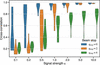Figure 10
Effect of beamstop size and noise level on reconstruction performance. Each violin plot shows the distribution of CC between reconstructed and ground-truth electron densities across all test proteins for different SNRs η.

As expected, progressively removing low-frequency information detrimentally affects performance. With $[q_{\rm {stop}} = 4]$ , the average CC drops significantly across all noise levels, failing to exceed 0.9 even at $[\eta = 10]$ . This underscores the critical role of low-frequency signals in establishing the contrast needed for an initial molecular envelope, which subsequently facilitates full structural recovery. Nevertheless, under these challenging conditions, reconstructions with large η still preserve meaningful electron density. Fig. 11 illustrates this by comparing three reconstructions of varying fidelity; specifically, panel (c) shows that the reconstruction generated with $[q_{\rm {stop}} = 4]$ and $[\eta = 10]$ retains clear structural similarity to the true density in panel (a).

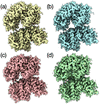Figure 11
Different reconstructions of protein GH168 using the magnitude-and-gradient algorithm. All images are plotted at a contour level of RMSD = 1, i.e. (Mean + 1 standard deviation), using ChimeraX. (a) The ground truth. All reconstructions are performed without a shrinkwrap support constraint. (b) $[q_{\rm {stop}} = 2,\eta = 10]$ , CC = 0.95. (c) $[q_{\rm {stop}} = 4,\eta = 10]$ , CC = 0.85. (d) $[q_{\rm {stop}} = 2,\eta = 1]$ , CC = 0.79.

While Fig. 10 establishes that the absence of central low-frequency data severely limits reconstruction quality, Fig. 12 demonstrates how real-space support constraints can effectively mitigate this loss. As discussed in the Introduction, approximate molecular envelopes are frequently obtainable from complementary low-resolution methods. By enforcing this prior spatial knowledge, the algorithm successfully recovers structures that otherwise fail to converge. To quantify this improvement, we tested two constraint levels: a `tight' envelope that closely matches the actual molecular boundary, and a `rough' envelope that includes the molecule alongside half of the surrounding solvent density. As noted by Kingston & Millane (2022), it is plausible to obtain an approximate support from low-resolution reconstructions. The results demonstrate that introducing real-space support constraints enables the recovery of structures that otherwise fail to converge.

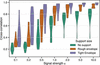Figure 12
Influence of real-space support constraints on reconstruction accuracy at different noise levels. Violin plots show CC distributions for reconstructions performed without a support (green), with a rough molecular envelope including partial solvent density (orange) and with a tight envelope closely matching the true molecular shape (purple). All simulations were conducted with $[q_{\rm {stop}} = 4]$ .

While loss of central intensities previously limited reconstruction quality, the inclusion of even approximate support constraints partly restores this information. For $[\eta]$ values of 5 and 10, a rough envelope is sufficient to improve the reconstruction to high levels. With a tight envelope, good reconstructions appear at values as low as an $[\eta]$ of 2 and interpretable features remain recoverable down to $[\eta = 0.5]$ . These results demonstrate that even approximate molecular envelopes – such as those obtainable from low-resolution data – can significantly enhance reconstruction robustness in challenging experimental conditions. This improvement arises because the support constraint effectively limits the search space for the electron density, compensating for the missing low-frequency information.

5. Conclusion

The magnitudes of structure factors obtained from the intensities measured at reciprocal-lattice points of a crystal are insufficient to uniquely determine the electron density within the unit cell. The unmeasured phases can nevertheless be recovered if more than 75% of the unit-cell electron density is known, as in macromolecular crystals with solvent fractions exceeding 75%. In such cases, IPR algorithms have been shown to be effective (Kingston & Millane, 2022; Fu et al., 2024). We investigated an approach proposed by Elser (2013), in which ab initio phase retrieval is performed using both diffraction intensities and their gradients at reciprocal-lattice points. These additional measurements increase the number of independent constraints and exceed the number of unknown variables required to describe the molecular electron density, even in the absence of significant solvent volume. The benefit of adding the gradients can be understood in considering the Patterson function obtained from the Bragg intensities. This real-space function repeats with the same periodicity as the unit cell and hence cannot capture the full range of distance pair correlations of the unit cell – it represents an aliased autocorrelation function of the electron density. The gradient information provides versions of the Patterson function weighted by the coordinate, allowing the aliasing to be unraveled.

We performed tests of Elser's approach on simulated diffraction data of protein crystals to determine the possibility of obtaining model-free electron-density reconstructions. These simulations included the extraction of intensity gradients from Bragg peaks of non-negligible width, as expected in serial crystallography measurements of nanocrystals (Spence et al., 2011) or from a crystal with a finite lattice correlation length. The simulations further incorporated experimentally relevant conditions, including low solvent fraction, missing low- $[{\bf q}]$ data and realistic noise models. The results demonstrate that the magnitude-and-gradient algorithm performs robustly across a wide range of solvent fractions and remains resilient even under high levels of noise, thereby supporting its potential application to experimental nanocrystal data. The algorithm successfully reconstructs electron densities even when low-frequency data are missing due to a beamstop.

The approach is well suited to the analysis of diffraction measurements acquired using modern X-ray free-electron lasers and fourth-generation synchrotron radiation facilities, where nanocrystal diffraction patterns often exhibit Bragg peaks spanning multiple pixels, enabling measurement of intensity gradients (Mendez et al., 2020 ).

Despite these results, the current implementation remains restricted to crystals with P1 symmetry, that is, to purely translational symmetry, and several limitations should be kept in mind, even for this scenario. First, the unwrapping function was fixed at its ground-truth form throughout. Elser (2013) found reconstructions to be only weakly sensitive to estimating it during the iteration, yet we have not tested this further. Second, we also assumed our coordinate system to be aligned with the reciprocal-lattice vectors, which is generally not the case in practice, requiring the additional treatment discussed at the end of Section 2.

More generally, the non-Bragg signal exploited here arises from the places where the crystal's periodic order is interrupted. Such regions are more likely to be disordered than the bulk, and because they are also where the exploited signal originates, they have an outsize effect on it. With higher crystallographic symmetry present, a disordered or reconstructed surface or a void can locally favor different unit cells, so that the measurement averages over several distinct cells that must then be disentangled. Even in the P1 case, where every coherent sub-volume encodes a molecule of the same orientation, the object itself may be distorted by surface effects or a disordered solvent shell or other effects, which could affect the measured gradients.

Future work should focus on improving the extraction of reliable intensity gradients and on applying the method to experimental nanocrystal data. Furthermore, the magnitude-and-gradient approach could be naturally integrated with complementary phasing strategies, such as the program by Kingston & Millane (2022), which leverages molecular envelopes derived from low-resolution data to further constrain the solution space. Extending the formalism to crystals with rotational symmetry remains an open challenge, since their termination can no longer be captured by a single scalar shape function and instead requires a description that accounts for the different symmetry-related copies at the crystal surface.

APPENDIX A

From constraints to projections

A1. The Fourier constraint – the divide projection

In the following derivation, the steps of Elser (2013) in Section 4.1.2 are retraced with supplementary details to clarify the progression. Note: in the original publication, the notation $[{\bf G}({\bf q})]$ is used instead of $[\nabla_{j}F({\bf q})]$ . The relationship between these notations is given by $[\nabla F({\bf q}) = 2\pi i{\bf G}({\bf q})]$ . Consequently, the real-space definitions of $[{\bf R}]$ also differ by a factor of $[2\pi i]$ . The variable σ is retained explicitly throughout the following derivation, as it acts as a tunable hyperparameter.

To jointly satisfy the constraints in equation (9) and equation (12) via a distance-minimizing step, the distance between $[{\bf F}^{(k)}]$ and $[{\bf F}^{(k+1)}]$ must first be minimized under the L2 norm, given by

$[\eqalignno{\Delta^{2} &= \sum_{q}|F^{(k+1)}({\bf q})-F^{(k)}({\bf q})|^{2}&\cr &\quad +\sigma^{2} \sum_{q}\sum_{j}|(\nabla_{j}F)^{(k+1)}({\bf q})-(\nabla_{j}F)^{(k)}( {\bf q})|^{2},&(27)}]$

where σ represents the scaling parameter between intensities and intensity gradients. The objective is to establish a projection from $[{\bf F}^{(k)}({\bf q})]$ to $[{\bf F}^{(k+1)}({\bf q})]$ by utilizing a Lagrange-multiplier-augmented distance. In the following formulation, the update for each $[{\bf F}^{(k+1)}({\bf q})]$ relies exclusively on information from the corresponding $[{\bf F}^{(k)}({\bf q})]$ and $[I({\bf q})]$ , independent of other reciprocal-space positions. For notational clarity, the explicit $[{\bf q}]$ dependence is therefore omitted.

Because the Fourier constraints are highly nonlinear, F^(k) and F^(k+1) are initially assumed to be fixed. A stationary point is then sought with respect to each $[(\nabla_{j}F)^{(k+1)}]$ in the Lagrange-multiplier-augmented distance. Holding F^(k+1) constant leaves the following expression to be minimized:

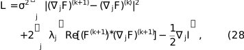
$[\eqalignno{{\cal L}& = \sigma^{2}\sum_{j}|(\nabla_{j}F)^{(k+1)}-(\nabla_{j}F)^{(k)}|^{2}&\cr &\quad + 2\sum_{j}\lambda_{j}\left\{{\rm Re}[{(F^{(k+1)})^{*}}(\nabla_{j}F)^{(k+1)}]- {{1} \over {2}}\nabla_{j}I\right\},&(28)}]$

where a real-valued Lagrange multiplier $[\lambda_{j}]$ is introduced for each axis j. This expression is minimized for the gradients $[(\nabla F)_{j}^{(k+1)}]$ by setting the derivative $[\delta{\cal L}/\delta(\nabla_{j}F)^{(k+1)} = 0]$ , leading to the update rule

$[(\nabla_{j}F)^{(k+1)} = (\nabla_{j}F)^{(k)}-{{\lambda_{j}} \over {\sigma^{2}}}F^{(k+ 1)}.\eqno(29)]$

Substituting this back into the constraint $[{\rm Re}[{(F^{(k+1)})^{*}}(\nabla_{j}F)^{(k+1)}] = {{1} \over {2}}\nabla_{j}I]$ and using $[|F^{(k+1)}|^{2} = I]$ , the multiplier is obtained as

$[\lambda_{j} = {{\sigma^{2}} \over {I}}\left\{{\rm Re}[{(F^{(k+1)})^{*}}(\nabla_{j}F) ^{(k)}]-{{1} \over {2}}\nabla_{j}I\right\}.\eqno(30)]$

Having formulated the gradient replicas $[(\nabla_{j}F)^{(k+1)}]$ , the stationary point of the total distance $[d(\varphi)]$ must be determined. Expanding the L2 norm components yields the total distance,

$[d(\varphi) = |F^{(k+1)}-F^{(k)}|^{2}+\sigma^{2}\sum_{j}|(\nabla_{j}F)^{(k+1)}-(\nabla_{j}F)^{(k)}|^{2}.\eqno(31)]$

The gradient distance term $[|(\nabla_{j}F)^{(k+1)}-(\nabla_{j}F)^{(k)}|^{2}]$ involves $[\{{\rm Re}[\sqrt{I}\exp(-i\varphi)(\nabla_{j}F)^{(k)}]\}^{2}]$ . The expansion of this square generates phase-independent terms, which are absorbed into the constant, and phase-dependent terms at frequencies φ and $[2\varphi]$ ,

$[\eqalignno{d(\varphi) &= -2{\rm Re}[a\exp({i\alpha})\exp({-i\varphi})]&\cr & \quad -2{\rm Re}[b\exp({i\beta})\exp({-i2 \varphi})]+{\rm const}.&(32)}]$

To determine the optimal phase φ of $[F^{(k+1)} = \sqrt{I}\exp(i\varphi)]$ , terms in equation (31) are grouped by $[\exp({i\varphi})]$ and $[\exp({2i\varphi})]$ . By substituting the condition $[|F^{(k+1)}|^{2} = I]$ , the first term expands as

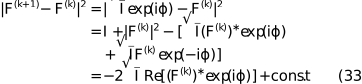
$[\eqalignno{|F^{(k+1)}-F^{(k)}|^{2} &= |\sqrt{I}\exp({i\varphi})-F^{(k)}|^{2}&\cr &= I+|F^{(k)}|^{2}-[\sqrt{I}{(F^{(k)})^{*}}\exp({i\varphi})&\cr &\quad+\sqrt{I}F^{ (k)}\exp({-i\varphi})]&\cr &= -2\sqrt{I}\ {\rm Re}[{(F^{(k)})^{*}}\exp({i\varphi})]+{\rm const}.&(33)}]$

Using the stationarity condition $[(\nabla_{j}F)^{(k+1)}-(\nabla_{j}F)^{(k)}]$ = $[-(\lambda_{j}/\sigma^{2})F^{(k+1)}]$ , the second term relates to the discrepancy between the expected and measured intensity gradients as follows:

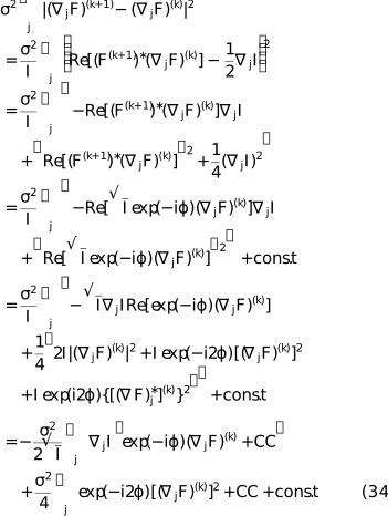
$[\eqalignno{&\sigma^{2}\sum_{j}|(\nabla_{j}F)^{(k+1)}-(\nabla_{j}F)^{(k)}|^{2}&\cr &= {{\sigma^{2}} \over {I}}\sum_{j}\left|{\rm Re}[{(F^{(k+1)})^{*}}(\nabla_{j}F)^{(k)}]-{{1} \over {2}}\nabla_{j}I\right|^{2}&\cr &= {{\sigma^{2}} \over {I}}\sum_{j}\Biggl(-{\rm Re}[{(F^{(k+1)})^{*}}(\nabla_{j}F)^{(k)}]\nabla_{j}I&\cr &\quad +\left\{{\rm Re}[{(F^{(k+1)})^{*}}(\nabla_{j}F)^ {(k)}]\right\}^{2}+{{1} \over {4}}(\nabla_{j}I)^{2}\Biggr)&\cr &= {{\sigma^{2}} \over {I}}\sum_{j}\Biggl(-{\rm Re}[\sqrt{I}\exp({-i \varphi})(\nabla_{j}F)^{(k)}]\nabla_{j}I&\cr &\quad +\left\{{\rm Re}[\sqrt{I}\exp({-i\varphi})(\nabla_{j}F)^{(k)}]\right\}^{2}\Biggr)+{\rm const.}&\cr &= {{\sigma^{2}} \over {I}}\sum_{j}\Biggl[-\sqrt{I}\nabla_{j}I{\rm Re }[\exp({-i\varphi})(\nabla_{j}F)^{(k)}]&\cr &\quad+{{1} \over {4}}\bigl(2I|(\nabla_{j}F)^{(k)}|^{2}+I\exp({-i2\varphi})[(\nabla_{j}F)^{(k)}]^{2}&\cr &\quad+I\exp({i2\varphi})\{[{(\nabla F)_{j}^{*}}]^{(k)}\}^{2}\bigr)\Biggr]+{\rm const.}&\cr &= -{{\sigma^{2}} \over {2\sqrt{I}}}\sum_{j}\nabla_{j}I\left[\exp({-i \varphi})(\nabla_{j}F)^{(k)}+{\rm CC}\right]&\cr &\quad+{{\sigma^{2}} \over {4}}\sum_{j}\exp( {-i2\varphi})[(\nabla_{j}F)^{(k)}]^{2}+{\rm CC}+{\rm const}. &(34)}]$

To solve for φ, terms that are linear in $[\exp({\pm i\varphi})]$ and terms that are quadratic [representing $[\exp({\pm i2\varphi})]$ ] are collected. To consolidate the expression, the complex constants $[a\exp({i\alpha})]$ and $[b\exp({i\beta})]$ are defined as

$[a\exp({i\alpha}) = \sqrt{I}F^{(k)}+{{\sigma^{2}} \over {2\sqrt{I}}}\sum_{j }\nabla_{j}I(\nabla_{j}F)^{(k)},\eqno(35)]$

$[b\exp({i\beta}) = -{{\sigma^{2}} \over {4}}\sum_{j}[(\nabla_{j}F)^{(k)}]^{ 2}.\eqno(36)]$

The distance function $[d(\varphi)]$ then takes the form of a non-convex potential:

$[d(\varphi) = -2a\cos(\varphi-\alpha)-2b\cos(2\varphi-\beta)+{\rm const}. \eqno(37)]$

Because the data constraint is nonlinear and nonconvex, the distance function may possess multiple stationary points. The core of the magnitude-and-gradient Fourier projection is the search for the argument that minimizes this potential. The optimal phase shift $[\psi = \varphi-\alpha]$ is defined as

$[\psi(c,\gamma) = {\rm argmin}_{\psi^{\prime}}[-\cos(\psi^{\prime})-c\cos(2\psi^ {\prime}-2\gamma)],\eqno(38)]$

where and $[\gamma = \beta/2-\alpha]$ . The final updated phase is then

$[\varphi = \alpha+\psi\left({{b} \over {a}},{{\beta} \over {2}}-\alpha\right).\eqno(39)]$

This phase is used to set $[F^{(k+1)} = \sqrt{I}\exp(i\varphi)]$ , which subsequently allows for the unique determination of the Lagrange multipliers $[\lambda_{j}]$ and the projected gradient replicas $[(\nabla_{j}F)^{(k+1)}]$ .

To summarize, the following projection is obtained to map from $[{\bf F}^{(k)}]$ to $[{\bf F}^{(k+1)}]$ satisfying the constraint set given by equation (9) and equation (12). The Fourier transform and its gradients are updated according to

$[\tilde{P}_{{\rm F,grad}}:\left\{\matrix{F^{(k+1)}\hfill & = \sqrt{I}\exp(i\varphi), \hfill\cr (\nabla_{j}F)^{(k+1)}& = (\nabla_{j}F)^{(k)}-({{\lambda_{j}} / {\sigma^{2}}})F^{(k +1)}.}\right.\eqno(40)]$

To apply this projection, $[a\exp(i\alpha)]$ and $[b\exp(i\beta)]$ are first determined via equation (35) and equation (36), respectively. Next, φ is calculated using equation (39) to update F^(k+1). Finally, $[\lambda_{j}]$ is evaluated via equation (30), allowing $[(\nabla_{j}F)^{(k+1)}]$ to be calculated.

Supporting information

Supporting figures S1 and S2. DOI: https://doi.org/10.1107/S1600576726008137/te5167sup1.pdf

Acknowledgements

We thank the members of the Institute for Algorithms and Complexity, of the CFEL Coherent Imaging Group and Rick Millane for their interesting comments and discussions. Open access funding enabled and organized by Projekt DEAL.

Funding information

We acknowledge Deutsches Elektronen Synchroton (DESY), a member of the Helmholtz Association, and DASHH, Data Science in Hamburg – Helmholtz Graduate School for the Structure of Matter, for financial support. Parts of this research were funded by and carried out at the Hamburg University of Technology.

References

Anscombe, F. J. (1948). Biometrika 35, 246–254. CrossRef Web of Science Google Scholar
Ayyer, K., Yefanov, O. M. & Chapman, H. N. (2018). X-ray Free Electron Lasers: a Revolution in Structural Biology, edited by S. Boutet, P. Fromme & M. S. Hunter, pp. 253–300. Cham: Springer International Publishing. Google Scholar
Ayyer, K., Yefanov, O. M., Oberthür, D., Roy-Chowdhury, S., Galli, L., Mariani, V., Basu, S., Coe, J., Conrad, C. E., Fromme, R., Schaffer, A., Dörner, K., James, D., Kupitz, C., Metz, M., Nelson, G., Xavier, P. L., Beyerlein, K. R., Schmidt, M., Sarrou, I., Spence, J. C. H., Weierstall, U., White, T. A., Yang, J.-H., Zhao, Y., Liang, M., Aquila, A., Hunter, M. S., Robinson, J. S., Koglin, J. E., Boutet, S., Fromme, P., Barty, A. & Chapman, H. N. (2016). Nature 530, 202–206. CrossRef PubMed Google Scholar
Barnett, M. J., Millane, R. P. & Kingston, R. L. (2024). Acta Cryst. D80, 800–818. CrossRef IUCr Journals Google Scholar
Berman, H. M., Westbrook, J., Feng, Z., Gilliland, G., Bhat, T. N., Weissig, H., Shindyalov, I. N. & Bourne, P. E. (2000). Nucleic Acids Res. 28, 235–242. Web of Science CrossRef PubMed CAS Google Scholar
Boyd, S., Parikh, N., Chu, E., Peleato, B. & Eckstein, J. (2011). Found. Trends Mach. Learn. 3, 1–122. CrossRef Google Scholar
Chen, J., Pande, K., Donatelli, J., Martin, A., Ayyer, K., Chapman, H., Bean, R., Schmidt, K. & Kirian, R. (2023). Ultramicroscopy 249, 113728. CrossRef PubMed Google Scholar
Chen, J. P. J., Donatelli, J. J., Schmidt, K. E. & Kirian, R. A. (2019). Acta Cryst. A75, 239–259. Web of Science CrossRef IUCr Journals Google Scholar
Elser, V. (2003). J. Opt. Soc. Am. A 20, 40. Web of Science CrossRef Google Scholar
Elser, V. (2013). Acta Cryst. A69, 559–569. Web of Science CrossRef CAS IUCr Journals Google Scholar
Elser, V. (2025). Solving Problems with Projections: From Phase Retrieval to Packing, pp. 187–233. Cambridge University Press. Google Scholar
Elser, V. & Millane, R. P. (2008). Acta Cryst. A64, 273–279. Web of Science CrossRef CAS IUCr Journals Google Scholar
Evans, P. & McCoy, A. (2008). Acta Cryst. D64, 1–10. Web of Science CrossRef CAS IUCr Journals Google Scholar
Fienup, J. R. (1982). Appl. Opt. 21, 2758. CrossRef PubMed Web of Science Google Scholar
Fu, R., Su, W.-P. & He, H. (2024). Crystals 14, 85. CrossRef Google Scholar
Gerchberg, R. W. & Saxton, W. O. (1972). Optik 35, 237–246. Google Scholar
Gravel, S. & Elser, V. (2008). Phys. Rev. E 78, 036706. CrossRef Google Scholar
Green, D. W., Ingram, V. M. & Perutz, M. F. (1954). Proc. R. Soc. London Ser. A 225, 287–307. CrossRef Google Scholar
Griffin, D. & Lim, J. (1984). IEEE Trans. Acoust. Speech Signal. Process. 32, 236–243. CrossRef Web of Science Google Scholar
He, H., Jiang, M. & Su, W.-P. (2019). Crystals 9, 55. CrossRef Google Scholar
Hendrickson, W. A. & Teeter, M. M. (1981). Nature 290, 107–113. CrossRef CAS PubMed Web of Science Google Scholar
Kingston, R. L. & Millane, R. P. (2022). IUCrJ 9, 648–665. CrossRef PubMed IUCr Journals Google Scholar
Kirian, R. A., Bean, R. J., Beyerlein, K. R., Barthelmess, M., Yoon, C. H., Wang, F., Capotondi, F., Pedersoli, E., Barty, A. & Chapman, H. N. (2015). Phys. Rev. X 5, 011015. Google Scholar
Luke, D. R. (2005). Inverse Probl. 21, 37–50. Web of Science CrossRef Google Scholar
Marchesini, S. (2007). Rev. Sci. Instrum. 78, 011301. Web of Science CrossRef PubMed Google Scholar
Marchesini, S., He, H., Chapman, H. N., Hau-Riege, S. P., Noy, A., Howells, M. R., Weierstall, U. & Spence, J. C. H. (2003). Phys. Rev. B 68, 140101. Web of Science CrossRef Google Scholar
Meisburger, S. P., Case, D. A. & Ando, N. (2020). Nat. Commun. 11, 1271. Web of Science CrossRef PubMed Google Scholar
Mendez, D., Bolotovsky, R., Bhowmick, A., Brewster, A. S., Kern, J., Yano, J., Holton, J. M. & Sauter, N. K. (2020). IUCrJ 7, 1151–1167. CrossRef PubMed IUCr Journals Google Scholar
Miao, J., Sayre, D. & Chapman, H. N. (1998). J. Opt. Soc. Am. A 15, 1662. CrossRef Google Scholar
Millane, R. P. (1990). J. Opt. Soc. Am. A 7, 394–411. CrossRef Google Scholar
Millane, R. P. (1993). J. Opt. Soc. Am. A 10, 1037–1045. CrossRef Google Scholar
Millane, R. P. & Lo, V. L. (2013). Acta Cryst. A69, 517–527. Web of Science CrossRef IUCr Journals Google Scholar
Morgan, A. J., Ayyer, K., Barty, A., Chen, J. P. J., Ekeberg, T., Oberthuer, D., White, T. A., Yefanov, O. & Chapman, H. N. (2019). Acta Cryst. A75, 25–40. Web of Science CrossRef IUCr Journals Google Scholar
Patterson, A. L. (1934). Phys. Rev. 46, 372–376. CrossRef CAS Google Scholar
Sayre, D. (1952). Acta Cryst. 5, 843. CrossRef IUCr Journals Web of Science Google Scholar
Shannon, C. (1949). Proc. IRE 37, 10–21. CrossRef Google Scholar
Spence, J. C. H., Kirian, R. A., Wang, X., Weierstall, U., Schmidt, K. E., White, T., Barty, A., Chapman, H. N., Marchesini, S. & Holton, J. (2011). Opt. Express 19, 2866–2873. CrossRef PubMed Google Scholar
Wen, Z., Yang, C., Liu, X. & Marchesini, S. (2012). Inverse Probl. 28, 115010. Web of Science CrossRef Google Scholar
Wojdyr, M. (2022). J. Open Source Software 7, 4200. Google Scholar

This is an open-access article distributed under the terms of the Creative Commons Attribution (CC-BY) Licence, which permits unrestricted use, distribution, and reproduction in any medium, provided the original authors and source are cited.

JOURNAL OF
APPLIED
CRYSTALLOGRAPHY

ISSN: 1600-5767

Volume 59| Part 6| December 2026|

https://doi.org/10.1107/S1600576726008137

Open

access

Format		BIBTeX
		EndNote
		RefMan
		Refer
		Medline
		CIF
		SGML
		Plain Text
		Text

Format		BIBTeX
		EndNote
		RefMan
		Refer
		Medline
		CIF
		SGML
		Plain Text
		Text

research papers\(\def\hfill{\hskip 5em}\def\hfil{\hskip 3em}\def\eqno#1{\hfil {#1}}\)

Iterative phase retrieval in macromolecular crystal diffraction using the gradients of intensities

1. Introduction

2. Measuring molecular intensity gradients

3. Algorithmic implementation

3.1. The unwrapping function

3.2. Reciprocal-space constraints

3.3. Fourier-space projection

Magnitude-only Fourier projection PF,mag

Magnitude-and-gradient Fourier projection PF,grad

3.4. Real-space constraints and projections

Real-space object projection PO,mag

Magnitude-and-gradient object projection PO,grad

3.5. Iterative projection algorithm

4. Results

4.1. Dependence on solvent fraction

4.2. Robustness to noise

5. Conclusion

APPENDIX A

From constraints to projections

A1. The Fourier constraint – the divide projection

Supporting information

Acknowledgements

Funding information

References

research papers

Magnitude-only Fourier projection P_F,mag

Magnitude-and-gradient Fourier projection P_F,grad

Real-space object projection P_O,mag

Magnitude-and-gradient object projection P_O,grad